Quantum Chaos Introduction

This web page is designed to introduce the basic concepts of quantum chaos and to provide an introduction to some of the research I have done. This page addresses the following main questions:

• What is chaos?
• What is quantum mechanics?
• What is Quantum Chaos?
• What kind of research have I done in quantum chaos?

Just follow the links to learn about each topic. Also, if you want to know even more about Quantum Chaos you can check out the Quantum Chaos Bibliography to find magazine articles and books about Quantum Chaos. Enjoy!

What is chaos?

The Laws of Motion discovered by Isaac Newton in the 17th Century made it possible to predict the motion of any particle once certain information about the particle is determined. The information that one must know in order to predict the particle’s motion consists of the following: the particle’s location in space, the particle’s speed and direction of motion (velocity), and the forces acting on the particle. Knowing the particle’s position and velocity seemed straightforward enough (although, as we shall see later, it is not), but the forces acting on the particle remained a mystery until Newton developed his theory of gravitation. Suddenly, there was a complete explanation of what seemed to be the most important force around: gravity. This appeared to be a major triumph. With the force of gravity explained, one could now predict the future of every particle once its position and velocity were specified. In theory this made it possible to determine the future of all matter, since all matter was thought to be composed of simple particles. The idea that the future could be predicted using Newton’s Laws is called determinism.

It was not until the 19th Century that solid evidence against this deterministic veiw was found. First of all, forces other than gravity (namely the electric and magnetic forces) had been discovered. Clearly there was more to understanding all of the forces acting on a particle than just understanding gravity. Further, Henri Poincare had shown that the behavior of even a small number of particles acting only under the force of gravity cannot be easily predicted. Poincare found that the motion of three or more particles under gravity can be quite complicated and although the motion is, in theory, exactly determined by Newton’s Laws and the force of gravity, in practice it cannot be predicted over long times. The problem is that the motion of such a system depends very sensitively on the initial positions and velocities of the particles involved. If one could specify these initial conditions with infinite accuracy then one could predict all of the future motion of the system (provided one had an infinite amount of time in which to do the calculation). In practice, though, one cannot know these initial conditions to infinite accuracy and it turns out that even very tiny errors in these values will lead to inaccurate prediction of the motion of the system after relatively short times.

More recently it has been found that many systems behave this way. With accurate initial conditions one can accurately predict the future motion for short times, but one can never predict the long-time behavior of the system. A system that has this property of unpredictability is referred to as chaotic. Chaos is defined mathematically as a situation in which the distance between two particles that start off in close to the same place, with close to the same velocity, increases exponentially with time. This property is referred to as “sensitive dependence on initial conditions” and it basically means that particles with nearly identical initial conditions can have drastically different motion as time goes on. This is the essence of chaos.

One way to distinguish between regular (non-chaotic) behavior and chaotic motion is by looking at a diagram called a Poincare surface of section (SOS). A SOS is a plot that shows the position (the x-coordinate of the plot) and velocity (the y-coordinate) of a particle at various times. This space that treats velocity as a coordinate along with position is called phase space. If the system has more than one spatial dimension then one must make a slice through the phase space (which has twice as many dimensions as the number of spatial dimensions: i.e. a 2D system has a 4-dimensional phase space) in order to create a 2D plot that can be printed on a page. In 1D systems that have forces that are periodic in time, one simply plots the position and velocity after each period. This type of SOS is called a strobe plot. Examples of strobe plots for a system with a mixed phase space (displaying both regular and chaotic behavior) are shown below. It is easy to distinguish between the regions of regular motion and the regions of chaotic motion. Regular motion appears as well-defined lines running through the phase space. Regions of chaotic motion, on the other hand, appear as a random jumble of points. Note that J denotes the velocity (or momentum) of the particle in the 1D system and the Greek letter Theta denotes the position.

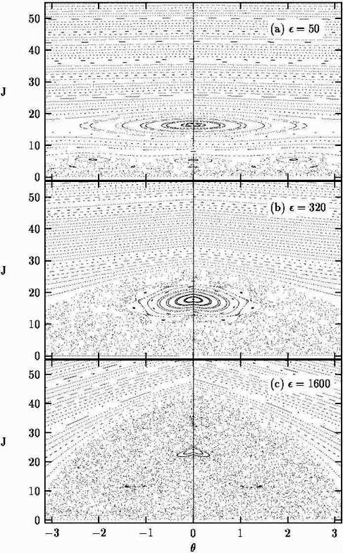The ellipse-shaped feature near J=20 in the plots is called a resonance. In a system where the forces are periodic in time, a resonance is a region of phase space where the natural period of motion in the system without the periodic forces is nearly equal to some integer multiple of the period of the forces. These resonances play and important role in the development of chaos in a system. In this system, the parameter denoted by the Greek letter epsilon controls the strength of the periodic forces. As the forces become stronger (epsilon is increased) the system becomes more chaotic as can be seen in the strobe plots shown here. This occurs because the system has several resonances. In figure (a) there is a chain of three elliptical “islands” visible near J=5. This is another resonance, in addition to the larger resonance near J=16. As the forces become stronger these resonances get larger. Wherever two resonances overlap a region of chaotic motion will be created. Thus, as the strength of the periodic forces is increased all of the resonances grow, overlap, and produce a large region of chaotic motion as seen in figure (c). This is essentially how chaos comes into being in systems like this. For other kinds of systems (e.g. systems with more than one spatial dimension, or systems without periodic forces) the details are different but the basic phenomenon is the same.

Now that you’ve been introduced to chaos in classical (i.e. Newtonian) systems, it is time to take a look at the strange world of Quantum Mechanics.

What is Quantum Mechanics?

Quantum mechanics is a theory developed in the early 20th Century to explain the behavior of atoms and other extremely small systems. Initially the theory used the ideas of classical (Newtonian) mechanics to explain several features exhibited by the hydrogen atom. In addition to the rules of classical mechanics, there was one extra rule that was “tacked on”. The extra rule said that a certain property, called the “action”, of a closed path for a classical particle must be an integer multiple of a constant called “h-bar”. Basically, the idea is that if a particle (like an electron in an atom) travels in a circle then that circular path must have an action equal to h-bar, or 2 h-bar, or 3-hbar, etc. This turned out to be sufficient to explain the hydrogen atom, but it could not explain many other atomic phenomena.

Eventually, a new theory was developed that could account for all of the observed atomic phenomena. This theory came in two different forms: one described an atomic system using something called a wave function, the other described the system using matrices. The two versions turn out to be equivalent to each other. In addition to providing a mathematical way to describe an atomic system, this new theory also provided a set of rules to determine the behavior of the quantum system in much the same way that Newton’s Laws determine the behavior of a classical system. However, this new theory of quantum mechanics is by no means equivalent to Newton’s Laws. There are some major differences between classical and quantum mechanics, and these differences are important for our discussion of quantum chaos.

Major Differences Between Newton’s Laws and Quantum Mechanics

1. In classical mechanics a particle can have any energy and any speed. In quantum mechanics these quantities are quantized. This means that a particle in a quantum system can only have certain values for its energy, and certain values for its speed (or momentum). These special values are called the energy or momentum eigenvalues of the quantum system. Associated with each eigenvalue is a special state called an eigenstate. The eigenvalues and eigenstates of a quantum system are the most important features for characterizing that systems behavior. There are no eigenvalues or eigenstates in classical mechanics.
2. Newton’s Laws allow one, in principle, to determine the exact location and velocity of a particle at some future time. Quantum mechanics, on the other hand, only determines the probability for a particle to be in a certain location with a certain velocity at some future time. The probabilistic nature of quantum mechanics makes it very different from classical mechanics.
3. Quantum mechanics incorporates what is known as the Heisenberg Uncertainty Principle. This principle states that one cannot know the location AND velocity of a quantum particle to infinite accuracy. The better you know the particle’s location, the more uncertain you must be about its velocity, and vice versa. In practice, the level of uncertainty that is required is so small that it is only noticeable when you are dealing with very tiny things like atoms. This is why we cannot see the effects of the Uncertainty Principle in our daily lives.
4. Quantum mechanics permits what are called “superpositions of states”. This means that a quantum particle can be in two different states at the same time. For instance, a particle can actually be located in two different places at one time. This is certainly not possible in classical mechanics.
5. Quantum mechanical systems can exhibit a number of other very interesting features, such as tunneling and entanglement. These features also represent significant differences between classical and quantum mechanics, although they will not be as important in our discussion of quantum chaos.

That is a pretty brief introduction to the ideas of quantum mechanics and many important features have been skipped. But the ideas presented above should make it clear that quantum mechanics is very different from classical (Newtonian) mechanics. We have seen how chaos is defined in classical mechanics. Can chaos also be defined in quantum mechanics? If so, how? We will explore this quesiton in the next section.

What is Quantum Chaos?

We have seen that quantum mechanics is very different from classical mechanics. So far we have only defined chaos in the context of classical mechanics. Is it possible to define chaotic behavior in the context of quantum mechanics? That question turns out to be a difficult one.

First of all, it is clear that one cannot define chaos in quantum mechanics the same way that it is defined in classical mechanics. The classical definition of chaos relies upon the ideas of sensitive dependence on initial conditions and exponentially diverging trajectories. This type of definition is simply not possible in quantum mechanics. To begin with, the Uncertainty Principle prevents us from talking about initial conditions in quantum mechanics since we cannot know the position and velocity of a particle simultaneously. Furthermore, the same principle prevents us from talking about trajectories in quantum mechanics because a trajectory is nothing more than a complete description of the position and velocity of a particle at all times. With these restrictions, one cannot talk about sensitive dependence on initial conditions or exponentially diverging trajectories in quantum mechanics. Those ideas simply don’t make sense in the context of the quantum theory. Thus, it is impossible for a quantum system to exhibit chaotic behavior if one uses the classical definition of chaos.

The probabilistic nature of quantum mechanics also makes it difficult to talk about chaos in the context of the quantum theory. Chaos is all about unpredictability, but unpredictability is built right into the foundation of quantum mechanics. One can never predict the exact behavior of a quantum system. One can only predict the probability that a quantum particle will behave in a certain way. So we are faced with a difficult choice. We can define chaos as it is defined in classical mechanics, in which case there is no chaos in quantum mechanics. Or we can define chaos in a vague way as “unpredictability”, in which case all of quantum mechanics is chaotic. Neither of these choices are very appealing. Fortunately, there are other alternatives.

One approach is to study how classical mechanics arises from quantum mechanics. Since all tiny particles must follow the rules of quantum mechanics, and since all matter is thought to be composed of tiny particles, the rules of classical mechanics that are followed by large objects must somehow arise from the rules of quantum mechanics. There is some very interesting research being done in this area, particularly in regard to the theory of decoherence. It may be that decoherence explains how chaotic classical motion can arise from non-chaotic quantum behavior. However, this does not give us a way to define chaos in quantum mechanics. It simply tells us that we need not be concerned if there turns out to be no chaos in quantum mechanics. We can still have chaos in classical mechanics if that is the case.

Another approach to the problem of quantum chaos is to formulate a probabilistic description of classical mechanics and attempt to find a definition of chaos that works in this new context. Instead of looking at individual trajectories in classical mechanics, one can look at a collection of a very large number of trajectories. One then examines how this collection evolves as time goes by. Collections of trajectories in chaotic classical systems do evolve in a much more complicated way than do collections of trajectories in regular classical systems. It turns out that the probability distributions in a quantum system evolve in very similar ways. However, the Uncertainty Principle prevents the quantum distributions from exactly following the classical collection of trajectories. Some progress has been made in understanding the relationship between this probabilistic description of classical mechanics and quantum mechanics, but so far no one has come up with a good way to define chaos in quantum mechanics.

A third approach to the problem of quantum chaos is to ignore the question of defining chaos in quantum mechanics and instead concentrate on identifying features of a quantum system that correspond to chaos in a classical system. In this approach one does not worry about whether or not the quantum system is “chaotic”. Instead, one tries to determine whether or not quantum versions of classically chaotic systems behave differently from quantum versions of classically regular systems. A great deal of progress has been made along these lines in recent years. For example, it has been discovered that the eigenvalues of a chaotic quantum system (the quantum version of a classically chaotic system) have different statistical properties than do the eigenvalues of a regular quantum system (the quantum version of a classically regular system). Another interesting development is that the distribution of eigenvalues in a chaotic quantum system can be determined using information about periodic orbits (trajectories that repeat the same path over and over) of the classical system.

My research centers on this third approach to studying quantum chaos. In particular, I investigate properties of the eigenstates (as opposed to the eigenvalues) of a quantum system that relate to chaos in the classical version of the system. More details about my work can be found in the next section.

What kind of research do you do?

My research focuses on computational studies of quantum chaos. Some of the topics in which I am interested are listed below.

I. Constructing a Quantum Phase Space

We have already seen that one way to identify chaotic classical motion is by looking at the phase space of the classical system. Can one create a similar phase space for a quantum system? The answer is yes, sort of. We know that the best way to examine the behavior of a quantum system is to study the system’s eigenstates. However, since quantum mechanics is probabilistic we can only talk about the probability distribution of a quantum state. Unfortunately, we can’t even create a probability distribution for a quantum state in phase space, because of the Uncertainty Principle. A true probability distribution in phase space would tell us the probability for a particle to have a certain exact location and exact velocity. But the Uncertainty Principle prevents us from even knowing the exact location and velocity of a quantum particle, so it is impossible to determine such a probability.

There is one way around this problem. That is to create a coarse-grained probability distribution for the quantum state in phase space. Such a distribution is called a Husimi distribution and it is basically a probability distribution in which the probability has been “smeared out” on the scale of h-bar. This allows us to comply with the Uncertainty Principle and still get a pretty good idea of what the quantum state looks like in phase space. The small-scale details of the quantum state get washed out, but we can still see where the quantum state sits in the phase space. These Husimi distributions can then be compared to the classical phase space to determine whether or not a particular eigenstate is associated with chaotic or regular classical motion. Examples of Husimi distributions are shown below.

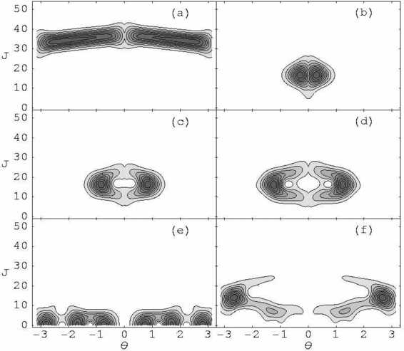This figure shows Husimi distributions for a variety of quantum eigenstates. These distributions should be compared with the classical phase space shown in part (b) of the figure in the section on classical chaos. It is clear that the Husimi distribution shown in (a) is associated with the region of regular motion near the top of the classical phase space. The Husimi distributions in (b), (c), and (d) are associated with the resonance region near J=16. The states shown in (e) and (f) are associated with the chaotic region of the classical phase space.

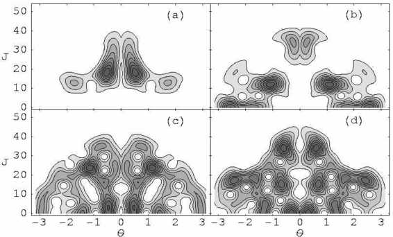The figure on the left shows Husimi distributions that should be compared to the classical phase space shown in part (c) of the figure in the section on classical chaos. These states are all associated with the region of classical chaos. Note that these states, particularly (c) and (d), are much more spread out than the “chaotic” states shown in parts (e) and (f) of the previous figure. This corresponds with the fact that the chaotic region in part (c) of the classical phase space figure is much larger in part (b).

II. Studying the Evolution of Quantum Eigenstates in a Chaotic System

In the section on classical chaos we learned how resonances cause regions of chaos to form and grow in the classical phase space. Now we have seen that quantum eigenstates can be associated with different regions of the classical phase space. We have also seen that these quantum state can become “more chaotic” (more spread out) as the classical phase space becomes more chaotic. In addition, we know that the statistics of the eigenvalue spectrum of a quantum system can change as the classical system becomes more chaotic. How do the eigenstates and eigenvalues of a quantum system undergo these changes?

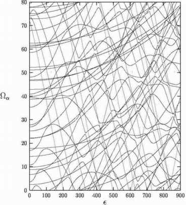The answer lies in a phenomenon known as an avoided crossing. In a time-periodic system (a system in which the forces are periodic in time), the eigenvalues of the quantum system change as the strength of the forces is increased and the system becomes more chaotic. It is observed that when two eigenvalues come close to each other in value, they will often repel each other. This phenomenon is called an avoided crossing. The figure to the right shows the eigenvalues of a quantum system (y-axis) as a function of the strength of the periodic forces (x-axis). Numerous avoided crossings can be seen. Note that the number of avoided crossings increases as the strength of the periodic forces is increased.

These avoided crossings are important because they are known to lead to changes in the statistical distribution of the eigenvalues. As the classical system becomes more and more chaotic, the quantum system has more and more avoided crossings and the statistical distribution of its eigenvalues changes. But what happens to the eigenstates when the quantum system has an avoided crossing? The answer depends on what type of avoided crossing occurs. Avoided crossings can be classified as sharp or broad, and the effect of an avoided crossing on the eigenstates of the quantum system depends on whether the avoided crossing is sharp or broad.

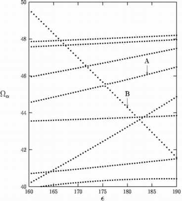
A sharp avoided crossing, like the one shown to the right, causes little change in the overall structure of the quantum eigenstates. In fact, what happens is that the two eigenstates whose eigenvalues are involved in the sharp avoided crossing simply exchange their structure as they pass through the avoided crossing.

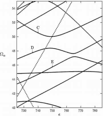
A broad avoided crossing, like the one shown to the left, does result in important changes to the structure of the eigenstates that are involved. After the system passes through the broad avoided crossing the eigenstates that were involved in the avoided crossing tend to be more spread out. This fits with our observation that Husimi distributions become more spread out as the classical system becomes more chaotic. Since there are three states involved in the broad avoided crossing shown here, we must follow the changes in the Husimi distributions of all three states.

Clearly avoided crossings play an important role in determining the evolution of quantum eigenstates as the classical system becomes increasingly chaotic. More research is needed to determine exactly how to distinguish between a sharp avoided crossing and a broad one, and to determine why these avoided crossings occur in the first place.

III. High Harmonic Generation

One of the reasons we have focused our study of quantum chaos on systems that have periodic driving forces is that these systems are the simplest systems that can exhibit classical chaos. Another reason, though, is that these systems exhibit a number of interesting phenomena that are associated with quantum chaos. One such phenomenon is high harmonic generation. High harmonic generation occurs because a charged particle will radiate light when it is driven by periodic forces. Usually, the light that is radiated is at a frequency equal to the frequency with which the particle is being driven. However, chaotic systems can radiate at integer multiples of the driving frequency, sometimes reaching frequencies over one hundred times greater than the driving frequency. This is known as high harmonic generation and it has many potential applications such as the development of inexpensive x-ray lasers. We have observed high harmonic generation in our simulations and we are seeking to understand the properties of a quantum system that lead to this phenomenon.

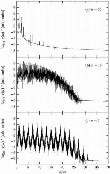The figure to the right displays some radiation spectra showing the radiation from various quantum states as a function of frequency. The spectrum in part (a) is from a state that sits in the regular region of the classical phase space and it produces radiation only at the driving frequency. The spectrum in part (b) is from a state that sits inside a classical resonance and it produces radiation at a number of frequencies but with no clearly defined harmonic peaks. The spectrum in part (c) is from a state that sits in the classical chaotic region of phase space. In this last spectrum there are well-defined harmonic peaks that produce significant radiation out to frequencies that are 19 times the driving frequency. This is an excellent example of high harmonic generation from a “chaotic” quantum state.

IV. Localization

Another interesting phenomenon displayed by periodically driven chaotic systems is localization. This occurs when a quantum state is confined to some small region of the phase space. In an open quantum system (a system in which the particle is free to travel out indefinitely, a phenomenon called ionization) localization may prevent or inhibit ionization because the quantum state is prevented from reaching an energy that would allow it to escape from the potential well and travel out to infinity. This localization can occur because the quantum state sits on a regular classical structure (like states (b), (c), and (d) from the first figure in this section, all of which sit on a classical resonance) in the phase space. However, it can also occur when the quantum state sits on an unstable periodic orbits (an orbit that repeats itself, but one where nearby trajectories are chaotic). This is known as non-classical localization (or quantum localization) and it is of great interest in atomic physics. We have identified a some states in a model system that are localized on unstable periodic orbits. Husimi distributions of these states are shown below.

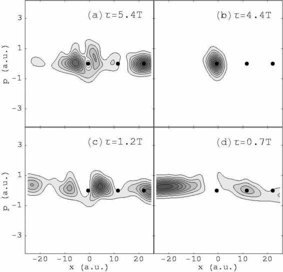The locations of periodic orbits are indicated by the black dots. The leftmost periodic orbit is stable and it is surrounded by a regular classical resonance. The other two periodic orbits, though, are unstable. Note that some of the Husimi distributions have peaks on or near the location of even these unstable periodic orbits. We have also found that the more strongly a quantum state is peaked on a periodic orbit, the less likely it is to ionize.

Still Want to Know More?

If you are interested in learning more about my work, please see the other Research links on my web page, as well as my Publications and Presentations page. You may also be interested in looking at some of the articles and books listed in the Quantum Chaos Bibliography.

Quantum Chaos Bibliography

Here is a list of articles and books that can help you learn about Quantum Chaos, along with some brief comments about each.

• Non-technical articles
  • “Quantum chaos”, R. V. Jensen, Nature 23 January 1992, p. 311. This is a great place to start and it is written by one of the leading researchers in the field.
  • “Quantum Chaos”, M. C. Gutzwiller, Scientific American January 1992, p. 78. Another good introduction written by a researcher who made on of the most exciting discoveries in the area of quantum chaos. Also see Gutzwiller’s book listed below.
  • “Quantum physics on the edge of chaos”, M. Berry, New Scientist 19 November 1987, p. 44. An early introduction to quantum chaos by an eminent physicist.
  • “Classical Mechanics, Quantum Mechanics, and the Arrow of Time”, T. A. Heppenheimer, MOSAIC Summer 1989, p. 2. Although not written by a researcher, this article provides a broad introduction to the work of several groups in the field.
• Technical textbooks
  • Chaos in Classical and Quantum Mechanics, M. C. Gutzwiller, Springer-Verlag, New York (1990). Focuses on the relation between quantum eigenvalues and classical periodic orbits, work done mostly by Gutzwiller himself.
  • The Transition to Chaos in Conservative Classical Systems: Quantum Manifestations, L. E. Reichl, Springer-Verlag, New York (1992). Contains a wealth of information. Written by my thesis advisor, so I may be a bit biased.
  • Quantum Signatures of Chaos, F. Haake, Springer-Verlag, New York (1992). Focuses on statistical properties of eigenvalues and their relation to chaos.
  • Quantum Chaos: An Introduction, H.-J. Stockmann, Cambridge University Press, Cambridge (2000). This is a new introduction to the subject that I have not yet had the chance to read.