Example homework problem:
You work for an automotive magazine, and you are investigating the relationship between a car’s gas mileage (in miles-per-gallon) and the amount of horsepower produced by a car’s engine. You collect the following data:
| Automobile: | 1 | 2 | 3 | 4 | 5 | 6 | 7 | 8 | 9 | 10 |
| Horsepower: | 95 | 135 | 120 | 167 | 210 | 146 | 245 | 110 | 160 | 130 |
| MPG: | 37 | 19 | 26 | 20 | 24 | 30 | 15 | 32 | 23 | 33 |
Is there a significant correlation between horsepower and MPG (alpha = .05)?
The goal of your analysis is to assess the naturally-occurring relationship between these two variables. To do this, we will compute the Pearson Product Moment Correlation Coefficient:
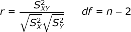 The correlation is equal to the ratio of the covariance between your variables to the variance within your variables. n is equal to the number of pairs of scores.
The Covariance between the two variables is equal to:
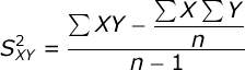 where ΣXY is equal to the sum of the crossproducts: you multiply each pair of scores and then add up the products.
Compute test statistic. Begin by computing the crossproduct scores, and then compute ΣXY, ΣX, and ΣY:
| Automobile: | 1 | 2 | 3 | 4 | 5 | 6 | 7 | 8 | 9 | 10 | Sum |
| Horsepower: | 95 | 135 | 120 | 167 | 210 | 146 | 245 | 110 | 160 | 130 | 1518 |
| MPG: | 37 | 19 | 26 | 20 | 24 | 30 | 15 | 32 | 23 | 33 | 259 |
| Crossproduct: | 3515 | 2565 | 3120 | 3340 | 5040 | 4380 | 3675 | 3520 | 3680 | 4290 | 37125 |
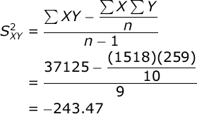
Here are the preliminary sums: ΣX = 1518, ΣY = 259, and ΣXY = 37125. n = 10.
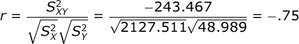
Compute the variance for each variable. You will find that the variance of X (horsepower) is equal to 2127.51, and the variance of Y (gas mileage) is equal to 48.99. If you would like help with these computations, see the documentation for descriptive statistics. Now, compute the covariance between the two variables:
 Let’s pause here for a moment, and place these three statistics into a Variance / Covariance Matrix:
| Variable: | Horsepower (X) |
MPG (Y) |
| Horsepower (X): | 2127.5111 | -243.4667 |
| MPG (Y): | 48.9889 |
where the values along the diagonal of the matrix are the variances of X and Y, and the value off the diagonal is the covariance between X and Y. It is a good habit to construct a variance/covariance matrix when you are working on correlation and regression problems.
Now that you have the variances and the covariance, you will find that the correlation is equal to:
 Conduct hypothesis test. Our correlation will have df equal to the number of pairs of scores minus 2. In our case, we have 10 automobiles, so we would have df = 10 – 2 = 8.
Alpha was set at .05 and we will conduct a two-tailed test. When you consult your table of critical values for r, you will find that if our obtained value of r is greater than .632, then we would conclude that the relationship between horsepower and gas mileage is significant — i.e., that r is significantly different from zero.
Since the obtained r (-.75) is greater in absolute value than the critical r (.632), we would conclude that there is a significant negative relationship between the horsepower level of the automobile and its gas mileage — i.e., the greater the horsepower, the lower the gas
mileage.
If you are not testing r directly in your class, then you are probably testing the significance of the correlation coefficient with the t distribution:
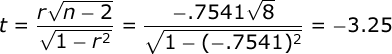 This t test will have df equal to n – 2, the same as r. In our case, df = 8. With alpha = .02 and assuming a two-tailed test, we would compare t to a critical value of 2.306.
Since our obtained t (-3.25) is greater in absolute value than our critical value of t (2.306), we would conclude that the correlation between horsepower and gas mileage was significant. Note that these two approaches are perfectly equivalent, and will always result in the same decision.
Effect Size. The correlation is an effective descriptive statistic in its own right. You know that it ranges from 0 to +1 and from 0 to -1, where 0 = no relationship and +1/-1 = perfect positive/negative relationship. In Statistical Power Analysis, Cohen suggested that we interpret a correlation of .10 as a small effect, a correlation of .30 as a moderate effect, and a correlation of .50 or greater as a large effect.
In addition, the square of the correlation (r²) is a very useful effect size estimate called the Coefficient of Determination. r² represents the proportion of variance in X and Y that is shared — i.e., the proportion of variance in one of the variables that can be accounted for by variation in the other variable. In our case, r² = -.7541² = .57. Thus, if you were predicting gas milage from horsepower, you could account for 57% of the variance in gas milage by variations in horsepower.