Your homework problem:
Aronson, Willerman, & Floyd (1966) investigated the impact of perceived competence on interpersonal liking. Participants were randomly assigned to one of four treatment conditions. In each, they listened to an audio recording of another student playing the part of a contestant on the ‘College Quiz Bowl’ game, where he would have to answer a number of interesting factual questions (similar to ‘Trivial Pursuit’). For half of the participants, the contestant was described as above average in every respect – he was an honor student, the editor of the campus yearbook, and a member of the school track team. For the other half of the participants, the contestant was described as average – he got average grades, he was a proofreader for the yearbook, and he tried out for the track team but did not compete. All the participants listened as the contestant played the Quiz Bowl game and answered many of the questions correctly (same male voice for all). For half of the participants, in the middle of one of his responses, the contestant spilled his coffee all over himself and sounded embarrassed about this accident. For the other half of the participants, the contestant did not spill his coffee. After the completion of the Quiz Bowl, the participants were asked to rate how much they liked the contestant – higher scores indicate greater interpersonal liking.
Here are some data similar to those collected by Aronson et al.:
| Ability Level |
Spilled Coffee | Did Not Spill Coffee |
| Average Ability | 2, 4, 5, 4, 3, 5 | 6, 4, 4, 5, 6, 3 |
| High Ability | 8, 6, 9, 7, 9, 8 | 6, 4, 5, 7, 3, 6 |
Did the manipulation of the contestant’s ability and whether or not he had an accident significantly affect the participants liking for him (alpha = .05)? Conduct a two-factor ANOVA to test the main effect for perceived competence of the contestant, the main effect for whether or not the contestant had an accident, and the interaction between the two factors.
The Analysis of Variance (ANOVA) for this design involves three independent F tests: one for the main effect of perceived ability level, one for the main effect of whether or not coffee was spilled, and one for the interaction between these two factors. Each F statistic is equal to the ratio of the Mean Square for one of the effects divided by the Mean Square Within Groups.
Compute the test statistic. The Source Table for this design will look like this:
| Source | SS | df | MS | F |
| Perceived Ability: | ||||
| Accident: | ||||
| Interaction: | ||||
| Within Groups: | ||||
| Total: |
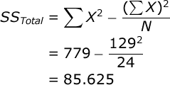
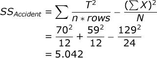
To get started, you should compute the following statistics: a) the sum of all scores (ΣX), the sum of all squared scores (ΣX²), and the overall number of scores (N), and the number of scores in each treatment group (n). In our case, ΣX=129, ΣX²=779, N=24, and n=6. Compute these statistics for yourself now.
Also, you should compute the sum of scores (T) for each treatment condition (cell) in this design:
| Ability Level |
Spilled Coffee |
Did Not Spill Coffee |
Row Total |
| Average Ability |
23 (n = 6) | 28 (n = 6) | 51 (12 scores) |
| High Ability |
47 (n = 6) | 31 (n = 6) | 78 (12 scores) |
| Column Total: | 70 (12 scores) | 59 (12 scores) | 129 (24 scores) |
Next, compute the total for each level of perceived ability (i.e., each row). Add these totals to your table. Also, compute the total for each level of the coffee spilling manipulation (i.e., each column). Again, add these to your table. Finally, compute the total of the row totals and the total of the column totals to make sure that this value is equal to the sum of your scores (ΣX=129).
Like the table above, your table should be displaying 9 totals: one for each cell (4), one for each row (2), one for each column (2), and one for all the scores. Important: take a minute at this time and note next to each total the number of individual scores that comprise that total. For each cell, this number is n. For each row total, this is equal to n times the number of columns. For each column total, this is equal to n times the number of rows. For the overall total, this is equal to N.
Now, we are ready to begin the Analysis of Variance. The Sum of Squares Total is equal to:
We need to compute the SS between all cells / treatment conditions. This will not be displayed in our Source Table, but it will be used to compute one of the SS statistics that is. Imagine that you have a one-factor design, and that you need to compute the SS
Between Groups:
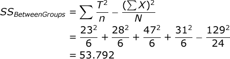
where T is equal to the sum of scores in a particular treatment group.
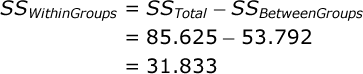
We can easily find the SS Within Groups by subtraction:
Now we will partition our between-groups variance into three systematic sources that characterize this design: the main effect for the first factor, the main effect for the second factor, and the interaction between the two factors.
We will begin by computing the SS for perceived ability level. Here, we focus on the row totals, and we ignore the column totals:
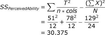
where T is equal to the row total. Next, we compute the SS for the spilling-coffee manipulation. Here, we focus on the column totals, and we ignore the row totals:
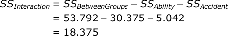
where T is equal to the column total. We find the SS for the interaction by subtraction:
Add each SS to your Source Table. The df Total is equal to the total number of scores minus one (N – 1). In our case this is: 24 – 1 = 23. The df Ability is equal to the number of levels of this factor minus one (a – 1). In our case this is: 2 – 1 = 1. The df Accident is equal to the number of levels of this factor minus one (b – 1). In our case this is: 2 – 1 = 1.
The df Within Groups is equal to the number of treatment conditions times (n – 1). In our case, this is: 4 * 5 = 20.
Each Mean Square (MS) is equal to the SS for that source divided by the df for that source. Each of the three F statistics is equal to the MS for an effect divided by MS Within Groups.
Here is your completed Source Table:
| Source | SS | df | MS | F |
| Ability: | 30.375 | 1 | 30.375 | 19.08 |
| Accident: | 5.042 | 1 | 5.042 | 3.17 |
| Interaction: | 18.375 | 1 | 18.375 | 11.54 |
| Within Groups: | 31.833 | 20 | 1.592 | |
| Total: | 85.625 | 23 |
Conduct hypothesis test. In our study, each of the the F statistics will have 1 and 20 df, and alpha = .05. If you look up the critical value of F in your table of critical values, you will see that if any of your obtained Fs is greater than 4.35, you would conclude that this effect was significant. You will see that this study resulted in a significant main effect for ability level, and a significant interaction between ability level and whether or not the contestant had an accident.
Explore significant interactions.Whenever a two-factor ANOVA results in a significant interaction effect, it is important to interpret the nature of that interaction. An interaction effect occurs when the effect that one o f your independent variables has on your dependent variable changes as a function of the level of the other independent variable. So, what does that mean in our study?
To find out, we need to explore the means of our treatment conditions. Divide the cell totals by n to compute the cell means:
| Ability Level |
Spilled Coffee |
Did Not Spill Coffee |
| Average | 3.83 | 4.67 |
| High | 7.83 | 5.17 |
Create a line graph of these cell means by hand, or you can use a program like Microsoft Excel® to create this graph:
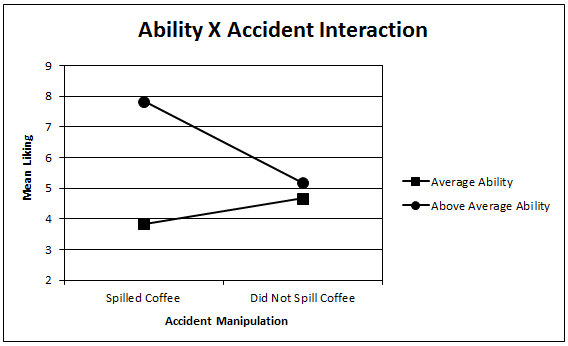
So what do the results tell us? We see that overall, we like the above- average contestant more than the average contestant (i.e., there was a main effect for perceived ability level). Also, this tendency to like the above-average contestant more than the average one is much stronger when the contestant spills his coffee (does something embarrassing) then it is when the contestant does not spill his coffee. Thus, the effect of perceived ability on liking depends on whether or not the contestant spilled their coffee. That is the nature of of the
interaction effect.
Compute effect size. You should compute the effect size for each of the three effects displayed in our Source Table. However, you will see that we can compute four different effect size statistics for each of our experimental effects. To illustrate these four approaches to computing effect size, we will focus only on the main effect for perceived ability. You can repeat these procedures to compute effect size for the other experimental effects
First, let’s compute Overall Eta Squared for the perceived ability effect, which is very simple:
![]()
Eta Squared is an estimate of the proportion of variance in your dependent variable that can be accounted for by the main effect of perceived ability level. However, the problem with
Eta Squared is that it will systematically over-estimate the variance accounted for in your experiment; the smaller the sample size in your study, the more biased Eta Squared will be. So, we typically prefer to compute an unbiased estimate of the variance accounted for. Here is how you compute Overall Omega Squared for the main effect of perceived ability level:
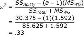 where a is the number of levels of ability (i.e., Factor A). So, we could conclude that our manipulation of of perceived ability level accounted for about 33% of the overall variance in the dependent variable (i.e., liking ratings). However, computing effect size for a factorial design is more complicated than it is for a one-factor design.
Some statisticians would argue that in this design, the variance due to the other main effect and that due to the interaction effect are not related to this main effect. They would suggest that we should partial out the variance from these two sources, and consider only the variance attributed to perceived ability level and within-group (i.e., error) variance when computing effect size.
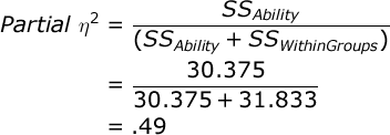
If we follow this approach, we would compute Partial Eta Squared:
…and Partial Omega Squared:
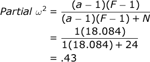
where (a – 1) is equal to the df for the ability factor. To help you check your computations, the table below displays all of the effect size statistics for this design:
| Source | Overall Eta Squared |
Overall Omega Squared |
Partial Eta Squared |
Partial Omega Squared |
| Ability: | .35 | .33 | .49 | .43 |
| Accident: | .06 | .04 | .14 | .08 |
| Interaction: | .21 | .19 | .37 | .31 |