Your homework problem:
You are interested in the effects of arousal on motor performance. A random sample of subjects perform a complex motor task under 3 conditions: no caffeine (low arousal), a small dose of caffeine (moderate arousal), and a large dose of caffeine (high arousal).
The dependent variable represents performance level: higher scores represent better performance.
This study resulted in the following data:
| Subject | Low Difficulty |
Moderate Difficulty |
High Difficulty |
| 1 | 15 | 17 | 19 |
| 2 | 2 | 7 | 4 |
| 3 | 11 | 12 | 6 |
| 4 | 13 | 15 | 5 |
| 5 | 12 | 12 | 7 |
| 6 | 2 | 18 | 11 |
| 7 | 8 | 12 | 5 |
| 8 | 9 | 14 | 2 |
Did the perceived level of caffeine significantly affect the participants’ performance (alpha = .05)? If your analysis reveals a significant overall effect, then make sure to explore all possible mean differences with a post-hoc analysis (same alpha).
The appropriate test statistic for your study would be the value of the F
statistic that would result from a One-Factor Repeated Measures Analysis of Variance (ANOVA):
![]()
The F statistic is equal to the ratio of the Mean Square
Treatment divided by the Mean Square Error. k is
equal to the number of groups, and n is equal to the number of
scores in each treatment condition (n is also equal to the number of
participants in your study).
Compute the test statistic. When we conduct an ANOVA, we typically
construct a Source Table
that details the sources of your variance and the corresponding degrees
of freedom:
| Source | SS | df | MS | F |
| Treatment: | ||||
| Subjects: | ||||
| Error: | ||||
| Total: |
To facilitate your ANOVA, you should compute the following statistics: a) the sum of all scores (ΣX), the sum of all squared scores (ΣX²), the overall number of scores (N), and the number of scores in each treatment group (n). In our case, ΣX=238, ΣX²=2964, N=24, and n=8. Compute these statistics for yourself now.
Also, you should compute the sum of scores (T) for each treatment condition:
| Low Arousal |
Moderate Arousal |
High Arousal |
|
| T: | 72 | 107 | 59 |
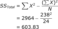
Now, you are ready to begin the Analysis of Variance. The Sum of Squares (SS) Total is equal to:
SS for the treatment conditions is equal to:
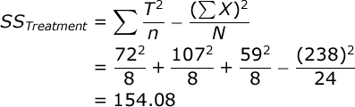
Again, T is equal to the sum of scores in a particular treatment group. Now, because this is a repeated-measures design, we need to compute the SS for subjects. We will begin by computing the total (T) for each subject in the study:
| Subject | Low Arousal |
Moderate Arousal |
High Arousal |
Total |
| 1 | 15 | 17 | 19 | 51 |
| 2 | 2 | 7 | 4 | 13 |
| 3 | 11 | 12 | 6 | 29 |
| 4 | 13 | 15 | 5 | 33 |
| 5 | 12 | 12 | 7 | 31 |
| 6 | 2 | 18 | 11 | 31 |
| 7 | 8 | 12 | 5 | 25 |
| 8 | 9 | 14 | 2 | 25 |
Once we have a T score for each subject, you compute SS for subjects:
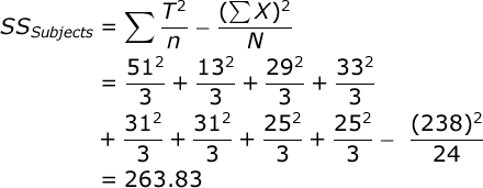
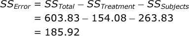
Now, we can find SS Error by subtraction:
Add these values to your Source Table. The df Total is equal to the total number of scores minus one (N – 1). In our case this is: 24 – 1 = 23. The df Treatment is equal to the number of treatment conditions minus one (k – 1). In our case this is: 3 – 1 = 2. The df Subjects is equal to the number of subjects minus one. In our case this is: 8 – 1 = 7. The df Error is equal to the number of treatment conditions minus one times the number of subjects minus one (k – 1)(n – 1). In our case, this is: 2 * 7 = 14.
Each Mean Square (MS) is equal to the SS for that source divided by the df for that source. In our case, MS Treatment = 154.08 / 2 = 77.042, and MS Error = 185.92 / 14 = 13.280.
Now you are ready to compute your test statistic. F is equal to:
![]()
Here is your completed Source Table:
| Source | SS | df | MS | F |
| Treatment: | 154.08 | 2 | 77.042 | 5.80 |
| Subjects: | 263.82 | 7 | ||
| Error: | 185.92 | 14 | 13.280 | |
| Total: | 603.83 | 23 |
Conduct hypothesis test. In our study, the F statistic will have 2 and 14 df, and alpha = .05. If you look up the critical value of F in your table of critical values, you will see that if your obtained F is greater than 3.74, you would conclude that perceived task difficulty significantly affected actual task performance (i.e., that there exists one or more mean differences among the treatment group means).
Since the obtained F (5.80) is greater than the critical value for F (3.74), you would conclude that there was a significant overall effect of perceived task difficulty on performance.
Compute effect size. We will compute the overall effect size two ways. First let’s compute Overall Eta Squared, which is very simple:
![]()
Eta Squared is an estimate of the proportion of variance in your dependent variable that can be accounted for by variation in your independent variable. However, computing effect size for a repeated-measures design is more complicated than it is for the completely-randomized design.
Some would argue that in this design, subject variance is a systematic source of variance that is not related to your hypothesis test. They would suggest that we should disregard subject variance and consider only treatment and error variance in our analysis. Thus, it would be more appropriate to compute effect size after we have removed subject variance from consideration.
If we follow this approach, we would compute Partial Eta Squared:
![]()
Computing Omega Squared -an unbiased estimate of effect size for the repeated-measures design is quite a journey. Here is the formula:
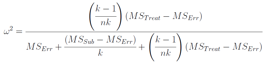
Yowza! We typically do not teach this formula in introductory courses. If you are feeling ambitious and you apply this formula to our data, you will find that Omega Squared for our results was .1988 ~ .20. Computing Partial Omega Squared is much easier, since the computations are based on the F statistic that you computed in your ANOVA:
![]()
Post-Hoc testing. The F statistic provides us with an omnibus test of whether or not our independent variable affected our dependent variable. It does not, however, help us to understand the exact nature of this effect.
In our case, we know that there exists at least one significant mean difference among our treatment groups, but we have no idea at this point which particular mean difference might be significant. So, we should follow up our ANOVA with a post-hoc test. We will examine all pair-wise comparisons among our treatment groups and figure out which treatment group mean differences are statistically significant.
We will employ Tukey’s Honestly Significant Difference (HSD) test (see note below). This will reveal to us what would constitute a statistically significant mean difference between any two treatment group means, controlling alpha over the course of all of these comparisons. In our study, an Honestly Significant Difference would be equal to: Unchanged: We will employ Tukey’s Honestly Significant Difference (HSD) test. This will reveal to us what would constitute a statistically significant mean difference between any two treatment group means, controlling alpha over the course of all of these comparisons. In our study, an Honestly Significant Difference would be equal to:
![]()
where q is equal to the Studentized Range Statistic and n is equal to the number of subjects. In our case, we have 8 subjects. When alpha is equal to .05, you have 3 treatment groups, and you have 14 df within-groups, when you examine your table of critical values, you will find that the critical value of the Studentized Range Statistic for this study is equal to 3.701. So, the value of a significant mean difference in this study would be equal to: Unchanged: where q is equal to the Studentized Range Statistic and n is equal to the number of subjects. In our case, we have 8 subjects. When alpha is equal to .05, you have 3 treatment groups, and you have 14 df within-groups, when you examine your table of critical values, you will find that the critical value of the Studentized Range Statistic for this study is equal to 3.701. So, the value of a significant mean difference in this study would be equal to:
![]()
Now, create a small table of the treatment group mean differences. Each value in this table is equal to the mean of the row group minus the mean of the column group:
| Treatment Group: | 1 | 2 | 3 |
| 1. Low: | -4.38 | 1.63 | |
| 2. Mod Diff: | 6.00 | ||
| 3. High Diff: | |||
We find that the mean difference between the moderate-difficult group and the high-difficulty group was significant. The other two mean differences were not significant.
Note. Using Tukey’s HSD test in this example assumes that your data demonstrate sphericity. Some would argue that we should not simply assume that sphericity is present, and that using Tukey’s test would not be appropriate for the repeated-measures design. However, since this example is specifically for illustrating hand computations and very basic statistical concepts, this test is the most feasible for us (and it’s results will be trustworthy if the sphericity assumption is met – you will see that the Bonferroni test resulted in the same outcome).
The most conservative and least controversial approach to post-hoc testing for this design involves computing a separate repeated-measures T test for each pairwise comparison. Then, we adjust the p value for each test according the number of tests being conducted (i.e., we multiply each p value by 3). This is called a Bonferroni adjustment. This would be easy to do if you are using a computer, and this is why that this approach is used by the Stats Homework software package. However, this approach would be a challenge to conduct by hand since you would have to compute three separate T tests and then have a special table for looking up the critical values of T.