One-Sample T Test

Example homework problem:

A car company claims that their Super Spiffy Sedan averages 31 mpg. You randomly select 8 Super Spiffies from local car dealerships and test their gas mileage under similar conditions.

You get the following Miles Per Gallon (MPG) scores:

Does the actual gas mileage for these cars deviate significantly from 31 (alpha = .05)?

If you would like help with the hand-written solution to this problem, click here.

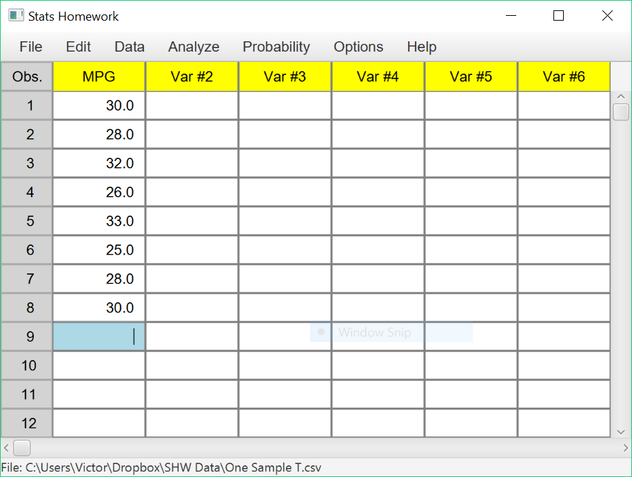
Enter these data into the first column of Stats Homework’s data manager and rename this variable. Your screen should look like this:

Make sure to double-check and save your data. To conduct your analysis, pull down the Analyze menu, choose One and Two Sample Tests, and then choose Z or T Test for One Sample.

You will be presented with a dialog window:

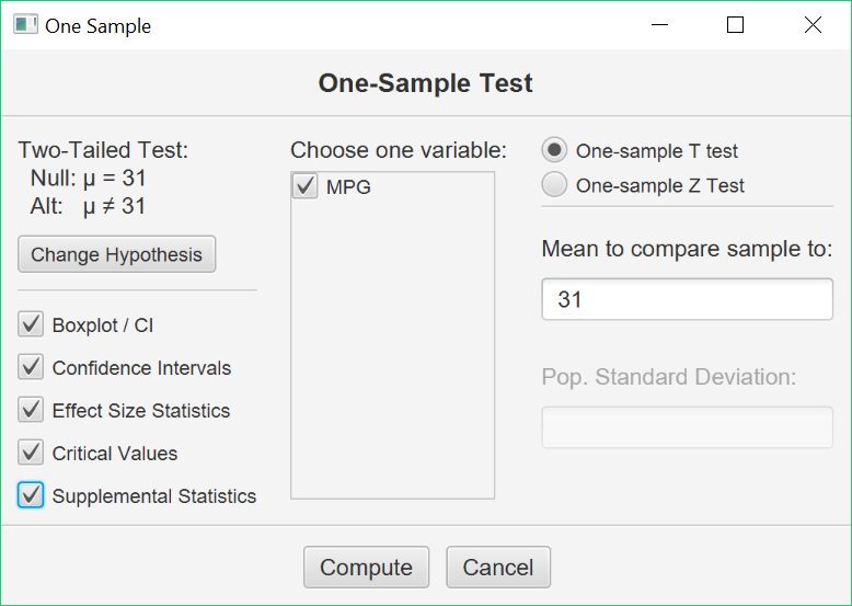
Enter 31 in the blank, and then check the variable that contains your data.  Select all the optional output, and click the Compute button.

Basic Output

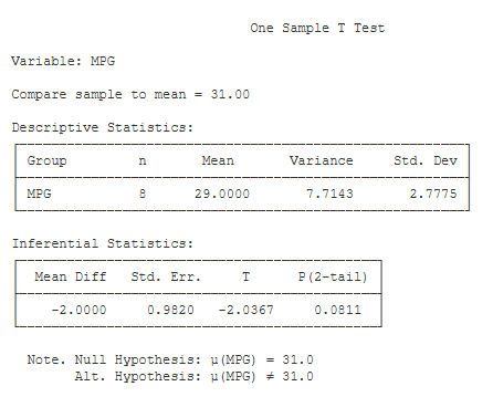
Compare Sample To. This is the population value that you are comparing the mean of your sample to with this T test. Double-check to make sure that you entered the correct value (31).

Descriptive Statistics. These basic statistics are described on the page for the explore procedure.

Inferential Statistics:

• Mean Diff (-2.00): this is equal to the mean of your sample minus the population value that you entered.
• Std. Err. (0.98): this is the Standard Error of your t Test. This will be equal to the standard deviation of your sample divided by the square root of the sample size.
• t (-2.04): this is the value of your test statistic. t is equal to the mean difference divided by the standard error.
• df (7): this is the df for your t test. df is equal to n – 1.
• p (2-tail) (.08): this is the chance probability / significance level for your t test if you are conducting a two-tailed or non-directional hypothesis test.

Optional Outputs

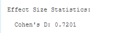
Effect Size Statistics.  Cohen’s D: (.72).  D is equal to the mean difference divided by the standard deviation of the sample. It standardizes the mean difference in terms of standard deviation units.

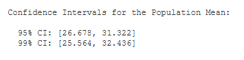
Confidence Intervals. You are given the 95% and 99% confidence intervals for the population mean, based on your sample mean. The 95% confidence interval tells you that, with 95% certainty, you would estimate the population mean to be between 28.68 and 33.32.

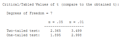
Critical Values. These are the values from a statistical table of critical values for the t test. In our case, we are conducting a two-tailed test with alpha = .05. So, we would compare the absolute value of our obtained t (2.04) to 2.365.

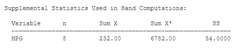
Supplemental Statistics Used in Hand Calculations. These are statistics that can be helpful if you would like to double check your hand-written computations.

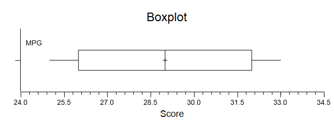
Box Plot.  Make sure to explore the options for this plot. You can change the scale, the title and labels, and the size of plot. You can also save this plot to disk or copy it to your clipboard.

See the Hand-Written Work

Return to Table of Contents