Example homework problem:

Twenty participants were given a list of 20 words to process. The 20 participants were randomly assigned to one of two treatment conditions. Half were instructed to count the number of vowels in each word (shallow processing). Half were instructed to judge whether the object described by each word would be useful if one were stranded on a desert island (deep processing). After a brief distractor task, all subjects were given a surprise free recall task. The number of words correctly recalled was recorded for each subject. Here are the data:

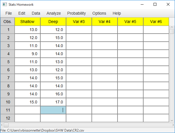
Shallow Processing:	13	12	11	9	11	13	14	14	14	15
Deep Processing:	12	15	14	14	13	12	15	14	16	17

Did the instructions given to the participants significantly affect their level of recall (alpha = .05)?

Note that these are the same data that we worked with when you were learning to use the independent t test procedure and the Mann-Whitney U procedure. This will allow you to compare and contrast the results of the permutation tests with these two traditional approaches.

---

We will use a separate variable approach.  Enter these data into the first two columns of Stats Homework’s data manager and rename the variables. Your screen should look like this:

Make sure to double-check and save your data. To conduct your analysis, pull down the Analyze menu, choose Permutation Tests, and then choose Two Independent Samples.

You will be presented with a dialog that will help you set up your analysis:

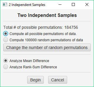
When you conduct a permutation test, the program will compute a criterion value from your sample data. In the case of two independent samples, you can choose the difference between the sample means if you consider your data to be interval — this test would be comparable to a t test. Or, you can use the difference between the sum of ranks for each sample if you consider your data to be ordinal — this test would be comparable to the Mann-Whitney U. The program will then create a number of permutations of your data and compute how often the permutations of your data meet this criterion.

Permutation tests can have one of two outcomes. You can find all possible permutations of your data and then compute the exact probability of obtaining a result as extreme as your criterion value. Or, you can find some number of random permutations of your data and then compute an estimated probability of obtaining a result as extreme as your criterion value.

To decide on which analysis to perform, you should consider how many permutations are possible. This value is displayed in the dialog window for this procedure. When you have two independent samples of n=10, there are 20! / (10! * 10!) = 184,756 possible different permutations of the data. This will not take very long on any modern computer, so computing the exact probability of your result would be a good choice.

So, for our first analysis, choose Compute all possible permutations of data and choose Analyze Mean Difference. This will allow us to compare the results of the permutation test to the results of a traditional t test.

Computing the Exact Probability of an Outcome

When you are ready, press the Begin button. While the permutation test is running, a progress bar will be displayed on the screen. In this case, the analysis will probably finish in only a second or two, and then it will produce the following output:

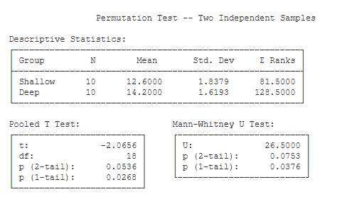
Descriptive Statistics. This table includes n, the mean, the standard deviation, and the sum of ranks for each group.

Pooled T Test. This table includes the results of submitting your data to a two-independent samples t test (with pooled variance).

Mann-Whitney U. This table includes the results of submitting your data to a Wilcoxon / Mann-Whitney U test.

Permutation Test.

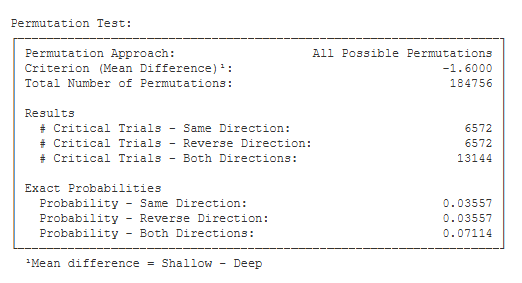
• Permutation Approach (All Possible Permutations): This will tell you whether you computed all possible permutations or some number of random permutations.
• Criterion (Mean Difference) (-1.60): This is the criterion used in this analysis — the difference between the sample means (i.e., 12.60 – 14.20).
• Total Number of Permutations (184756): This is the number of permutations computed.
• Results:
  • # Critical Trials – Same Direction (6572): This is the number of permutations that resulted in a mean difference equal to or greater than the criterion value in the
    same direction as the criterion value (i.e., -1.60).
  • # Critical Trials – Reverse Direction (6572): This is the number of permutations that resulted in a mean difference equal to or greater than the criterion value in the opposite direction as the criterion value (i.e., +1.60).
  • # Critical Trials – Both Directions (13144): This is the number of permutations that resulted in a mean difference equal to or greater than the criterion value in either
    direction.
• Exact Probabilities:
  • Probability – Same Direction (0.03557): This is the number of critical trials in the same direction as the criterion divided by the total number of permutations (i.e., 6572 / 184756).
  • Probability – Reverse Direction (0.03557): This is the number of critical trials in the opposite direction as the criterion divided by the total number of permutations (i.e., 6572 / 184756).
  • Probability – Both Directions (0.07114): This is the number of critical trials in either direction divided by the total number of permutations (i.e., 13144 / 184756).

Estimating the Probability of an Outcome

It is often the case that the total number of permutations of your data is quite large. You will find this to be especially problematic when you are working with research designs with more than two groups. For example, if you have a randomized design with 4 groups and n = 6 in each group, there are 2,308,743,493,055 possible permutations of your data. Unless you would like to wait a while for your analysis to finish (several weeks) , you will want to take a different approach to finding the probability of your outcome.

The Law of Large Numbers offers us a very reasonable compromise solution to this
problem. We can create a number of random permutations of our data and find the proportion of these random samples that meet our criterion. This will provide us an estimate of the chance probability of our outcome. The greater the number of random samples, the less variance our estimate of p will have.

With today’s computers, it is feasible to compute a relatively large number of random permutations in a relatively short period of time. For example, on my current computers, I can compute 1,000,000 random permutations of our data in about 3 seconds.

So, let’s estimate the chance probability of our results so that you will be ready to use this approach when it is more feasible. Again, pull down the Analyze menu, choose Permutation Tests, and then choose Two Independent Samples. You will again see this dialog window:

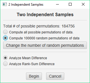
This time, choose Compute 100000 random permutations of data. This is the default number of random permutations for each of the permutation procedures. If you would like to compute more or less permutations, just press the Change the number of random permutations button and enter the number of permutations desired in the dialog window that is presented.

When you are ready, press the Begin button. This analysis will finish very quickly and produce an output page similar to that discussed earlier. The first three tables will be identical. Let’s focus on the results of the permutation test. Note that your results will not match exactly those below, but will be similar.

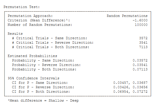
Permutation Test.

• Permutation Approach (Random Permutations): This will tell you whether you computed all possible permutations or some number of random permutations.
• Criterion (Mean Difference) (-1.60): This is the criterion used in this analysis — the difference between the sample means (i.e., 12.60 – 14.20).
• Number of Random Permutations (100000): This is the number of permutations computed.
• Results:
  • # Critical Trials – Same Direction (3572): This is the number of permutations that resulted in a mean difference equal to or greater than the criterion value in the same
    same direction as the criterion value.
  • # Critical Trials – Reverse Direction (3541): This is the number of permutations that resulted in a mean difference equal to or greater than the criterion value in the
    opposite direction as the criterion value.
  • # Critical Trials – Both Directions (7113): This is the number of permutations that resulted in a mean difference equal to or greater than the criterion value in either
    direction.
• Estimated Probabilities:
  • Probability – Same Direction (0.036): This is the number of critical trials in the same direction as the criterion divided by the total number of permutations (i.e., 3572 / 100000).
  • Probability – Reverse Direction (0.035): This is the number of critical trials in the opposite direction as the criterion divided by the total number of permutations (i.e., 3541 / 100000).
  • Probability – Both Directions (0.071): This is the number of critical trials in either direction divided by the total number of permutations (i.e., 7113 / 100000).
• 95% Confidence Intervals:
  • CI for P – Same Direction (0.035, 0.037): This is the 95% confidence interval for the estimate of the 1-tailed p value .
  • CI for P – Reverse Direction (0.034, 0.037): This is the 95% confidence interval for the estimate of the 1-tailed p value.
  • CI for P – Both Directions (0.070, 0.073): This is the 95% confidence interval for the estimate of the 2-tailed p value.

Learn More About Permutation Tests

To better understand the idea of estimating p, repeat this analysis several times. Note that your estimate of p will vary a bit from analysis to analysis. Also, vary the number of permutations — run this analysis a couple of times with 1,000 random permutations of your data, and then run your analysis a couple of times with 1,000,000 random  permutations of your data. Note the variation in your estimates of p and in your confidence intervals.

---

Return to Table of Contents