Example homework problem:
You work for an automotive magazine, and you are investigating the relationship between a car’s gas mileage (in miles-per-gallon) and the amount of horsepower produced by a car’s engine. You collect the following data:
| Automobile: | 1 | 2 | 3 | 4 | 5 | 6 | 7 | 8 | 9 | 10 |
| Horsepower: | 95 | 135 | 120 | 167 | 210 | 146 | 245 | 110 | 160 | 130 |
| MPG: | 37 | 19 | 26 | 20 | 24 | 30 | 15 | 32 | 23 | 33 |
Compute the best-fitting regression line (Y’ = a + bx) for predicting a car’s gas mileage from its horsepower. Test to see if the slope of this regression line deviates significantly from zero (alpha = .05).
The goal of your analysis is to predict the value of the outcome variable (Y: gas milage) given a value for the predictor variable (X: horsepower). To do this, we will compute the best-fitting regression line:
![]()
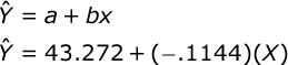
where the predicted value of Y is equal to the Y intercept (a) plus the product of a given value of X and the slope of the regression line (b).
We will begin our computations by computing the Variance/Covariance Matrix:
| Variable: | Horsepower (X) |
MPG (Y) |
| Horsepower (X): | 2127.5111 | -243.4667 |
| MPG (Y): | 48.9889 |
which presents the variance of X (2127.51), the variance of Y (48.99), and the covariance between X and Y (-243.47). The variable means have also been added. For help computing the variance and covariance, see the documentation for descriptive statistics and the documentation for correlation, respectively.
The slope of the regression line is equal to:
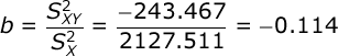
The slope of the regression line (b) is equal to the covariance between the two variables divided by the variance of the predictor variable (X).
Next, find the value of the Y intercept:
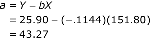
If you would like help computing the means, then see the documentation for descriptive statistics. Here is the completed regression equation:
Conduct hypothesis test. We would like to know if the value of b is significantly different from zero. There are several approaches. For example, we can use the t test for the slope:
![]()
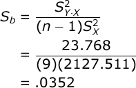
where b is the slope of the regression line, S(b) is the Standard Error of the slope, and n is the number of pairs of scores. The standard error of the slope is equal to:
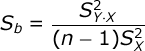
The numerator of this formula refers to the Variance of the Estimate. This is computed with this formula:
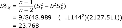
Now that you have computed the Variance of the Estimate, you can compute
the Standard Error of the Slope:
And now that you have the standard error of the slope, you can compute
the value of your t test:
![]()
Recall that the df for this t test is equal to n – 2, where n is the number of pairs of scores. So, our df is equal to 8.
Alpha was set at .05 and we will conduct a two-tailed test. When you consult your table
of critical values for t, you will find that if the absolute value of our obtained t is greater than 2.306, then we would conclude that the relationship between horsepower and gas mileage is significant — i.e., that the slope of the regression line is significantly different from zero.
Since the obtained t (-3.25) is greater in absolute value than the critical t (2.306), we would conclude that there is a significant negative relationship between the horsepower level of the automobile and its gas mileage — i.e., the greater the horsepower, the lower the gas mileage.
The Standardized Regression Coefficient. The problem with b is that it will vary greatly in value depending on the scales of X and Y. It is not a useful descriptive statistic at all. So, we will typically convert b to the Standardized Regression Coefficient (β):
![]()
The standardized regression coefficient is equal to the slope of the regression line predicting Y from X after you have converted both variables to Standard Scores (Z scores). When you have one predictor, β = r, the correlation coefficient. Think about it — the correlation coefficient is the slope of the regression line for predicting the Z of Y from the Z of X (in that case, the Y intercept will be 0). Don’t believe me? Convert both of your variables to Z scores and repeat your regression analysis — see how it turns out!
Now that you have r, you can easily compute r². r² = -.7541² = .57. This is the Coefficient of Determination; r² represents the proportion of variance in Y that can be accounted for by variation in X.
The Analysis of Variance. We will now cover another approach that you can use to see if the slope (b) of your regression line is significantly different from zero — the Analysis of Variance (ANOVA).
Our test statistic will be the value of the F statistic:
![]()
The F statistic is equal to the ratio of the Mean Square Due to Regression divided by the Mean Square Error. n is equal to the number of observations (i.e., the number of automobiles), and k is equal to the number of predictor variables (i.e., one: gas mileage).
Compute the test statistic. When we conduct an ANOVA, we typically construct a Source Table that details the sources of your variance and the corresponding degrees
of freedom:
| Source | SS | df | MS | F |
| Regression: | ||||
| Error: | ||||
| Total: |
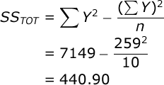
To facilitate your ANOVA, you should compute the following statistics: a) the sum of all of your outcome scores (ΣY), the sum of all squared outcome scores (ΣY²), and the number of observations (n). In our case, ΣY=259, ΣY²=7149, and n=10.
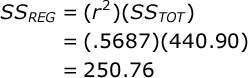
Also, you should keep handy the value of r² that we computed above (r² = .5687).
Now, you are ready to conduct an Analysis of Variance. The Sum of Squares (SS) Total is equal to:
The SS due to regression is equal to:
The SS error can be found by subtraction:
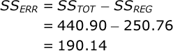
Add these values to your Source Table. The df Total is equal to the total number of observations minus one (n – 1). In our case this is: 10-1=9. The df Regression is equal to the number of predictors (k). In our case this is: 1. The df Error is equal to the number of observations minus two (n – 2). In our case this is: 10-2=8.
Each Mean Square (MS) is equal to the SS for that source divided by the df for that source. In our case, MS Regression = 250.76 / 1 = 250.76, and MS Error = 190.15 / 8 = 23.77. Note that MS Error is exactly equal to the Variance of the Estimate that we computed earlier — 23.678. That’s what MS Error means — error variance in our predictions.
Now you are ready to compute your test statistic. F is equal to:
![]()
Here is your completed Source Table:
| Source | SS | df | MS | F |
| Regression: | 250.755 | 1 | 250.755 | 10.55 |
| Error: | 190.145 | 8 | 23.768 | |
| Total: | 440.900 | 9 |
Conduct hypothesis test. In our study, the F statistic will have 1 and 8 df, and alpha = .05. If you look up the critical value of F in your table of critical values, you will see that if your obtained F is greater than 5.32, you would conclude that there is a significant relationship between X and Y (i.e., that a car’s horsepower is a significant predictor of the car’s gas mileage.
Since the obtained F (10.55) is greater than the critical value for F (5.32), you would conclude that there was a significant linear relationship between horsepower and gas mileage.
Effect Size. We already know that the correlation between horsepower and gas mileage (r) is equal to -.75, and that r² = .57. And, you know that r² represents the proportion of variance in Y that can be accounted for by variance in X. So, we can say that knowing the horsepower of cars allows us to account for 57% of the variance in the cars’ gas mileage scores.
However, the problem with r² is that it will systematically over-estimate the variance accounted for in your outcome variable; the smaller the sample size in your study, the more biased r² will be. So, we typically prefer to compute an unbiased estimate of the variance accounted for. There is a simple solution — we will compute Adjusted R²:
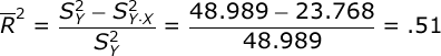
The numerator of this formula is equal to the variance in your outcome variable (Y) minus the Variance of the Estimate (or MS Error). Then, divide this difference by the variance of Y.
Notice that Adjusted R² will always be a smaller value than was r². We would conclude that using the horsepower of cars as a predictor variable can account for 51% of the variance in cars’ gas mileage.