To access this routine from within Stats Homework, pull down the Probability menu, select Illustrate Areas in a Distribution, and then select Illustrate Statistical Power with the Normal Distribution. If you are using the stand-alone program, you will not need to do this. Here is the user interface:
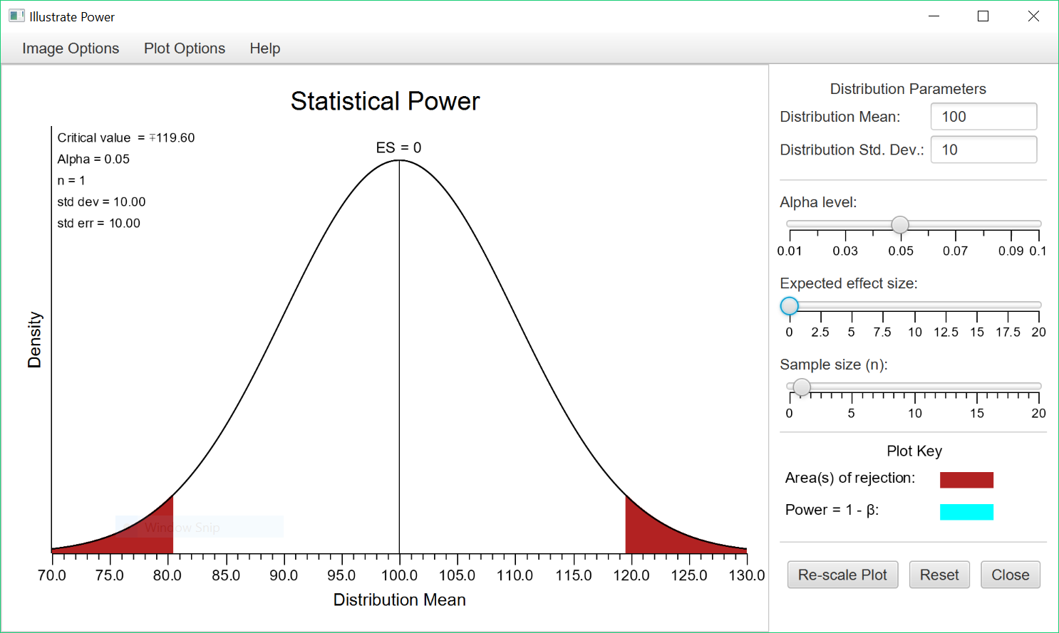
This program models the situation you face when you are conducting a null-hypothesis test using the normal distribution (e.g., a one-sample z test of the mean). The distribution you see above is a model of your null hypothesis — i.e., you start with the assumption that the effect size of your research is zero. The distribution you see here is a normal distribution with a mean of 100 and a standard deviation of 10.
If you were to get a result that falls in one of the red tails -the areas of rejection- you would reject your null hypothesis and conclude that your result represents a statistically-significant effect. The default is for you to assess a non-directional (i.e., two-tailed) hypothesis with an alpha = .05. So, the critical value of your z statistic would be +/- 1.96. This corresponds to a score of 119.60 in this distribution ([1.96 * 10] + 100 = 119.6).
Ok, let’s consider an effect size greater than zero. Move the effect-size slider back and forth, and then release it at 10.0. Then, press the “Re-scale Plot” button:
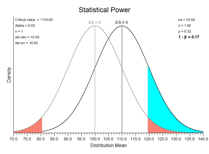 Notice that a new distribution appears with a mean of 110 (this is 100 plus your effect size of 10). This is a model of an alternative to your null — i.e., that your result comes from a distribution with a mean different from 100. If this were the result of your research, you would have obtained a z statistic value of 1.00: z = (research mean – null mean) / standard deviation = (110 – 100) / 10 = 1.0. If this were an actual research result, this z value (1.0) would not fall in the area of rejection (i.e., a z value greater than 1.96), so you would fail to reject the null hypothesis.
Imagine that you are randomly sampling results from this alternative distribution. Sometimes (17% of the time), the result you obtain would fall in the rejection area of the null distribution (this is the blue area highlighted in the graph). This area represents the statistical power of this test — the probability that you will reject the null hypothesis given that some alternative is actually true. This also tells us that 83% of the time, we will fail to reject the null. This is Beta — the probability that you fail to reject the null hypothesis when it is in fact false. Power is 1 – Beta.
In the above situation, you are working with single scores (i.e., n = 1). In most research situations, you will be working with some sample with n greater than 1. Slide the “n” slider back and forth, and see how this changes the shape of the distributions, and thus, the amount that they overlap. Notice that as n increases, the value of your z statistic increases, and the critical value required to reject your null hypothesis decreases. Slide this slider to 5 and release it. Then, press the “Re-Scale Plot” button:
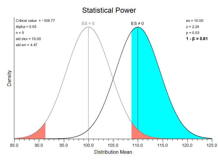 Here you can see that the effect size –the mean of the alternative distribution– is still 10.0 (1 standard deviation above the mean in a normal distribution). However, the standard error of the distributions is now 4.47. Standard error = standard deviation / sqrt(n) = 10.0 / sqrt (5) = 4.47. Now, the z statistic is 2.24. z is equal to (alternative mean – null mean) / standard error =(110 – 100) / (10.0 / sqrt(5)) = 2.24. If this were an actual research result this z statistic of 2.24 would fall in the area of rejection (a value greater than 1.96), which would lead you to reject the null hypothesis.
Now, the area of the alternative distribution that falls in the null’s rejection region is much greater — 61%. This illustrates one of the important dynamics of statistical power: given an effect size greater than zero, power will increase as you increase sample size, making it more likely that you reject the null.
Switch back and forth studying power (1 – Beta), and then the probability of making a Type II error (Beta). The option for this is found on the “Plot Options” menu. Also, switch back and forth between a two-tailed and a one-tailed hypothesis test. Side each of the sliders back and forth and study he effect that your action has on the blue area — the level of power in your research. You will learn about how each of these factors affect the level of statistical power in your research:
- Alpha Level: as alpha increases, so does the level of statistical power.
- Effect Size: as effect size increases, so does the level of statistical power.
- Sample Size: as n increases, so does the level of statistical power.
- One-tailed hypothesis tests have greater power than do two-tailed hypothesis tests.
Now that you understand how these factors can affect the power of your research, it is very important that you use this knowledge properly. You should always determine whether you are going to conduct a two-tailed or one-tailed test, and your level of alpha before you conduct a hypothesis test. And, it’s very important that you make these choices to pursue the greatest validity in your research and not simply to pursue the greatest statistical power. It is considered unethical to choose your test’s direction or alpha level after the fact in an effort to produce a statistically significant result.