This procedure is designed to support your learning of the Central Limit Theorem. It will randomly sample from a population and create sampling distributions. The population can be made up of random scores from a variety of different distributions, or it can be entered manually by the user.
To access this procedure, pull down the Probability menu, and then click Generate Sampling Distributions. Here is the dialog you will be working with:
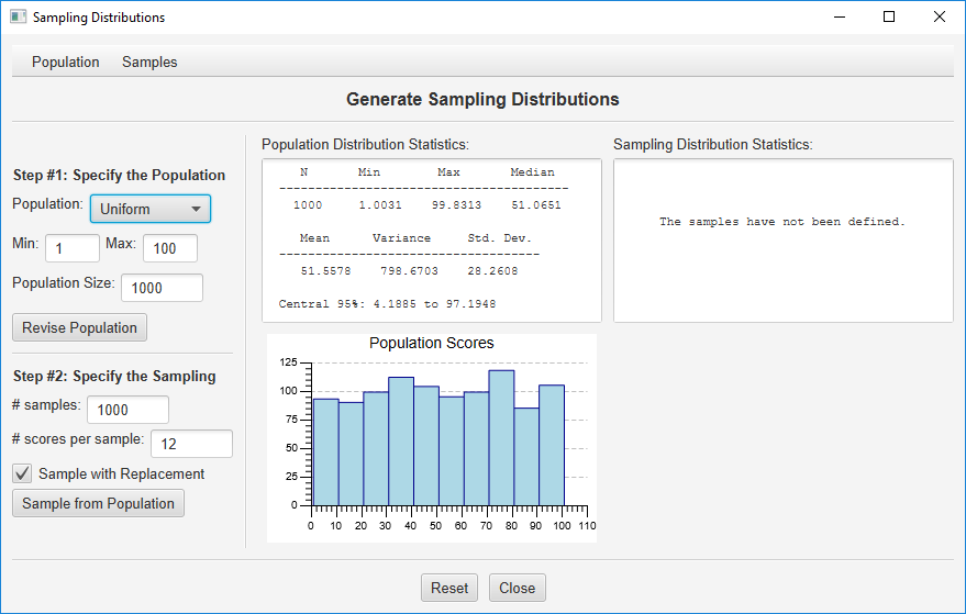
Step #1: Specify the Population. We will be taking random samples from a pre-defined population distribution of scores. This is specified by the options in the top half of the left column of the dialog, and the resulting population will be described in the center column. As you can see, the default is to randomly generate a population of 1,000 scores from a uniform distribution that has a minimum score of 1 and a maximum score of 100. Let’s start here; we will work with some alternative populations later.
Note that your population will have a mean and median close to 50, with a standard deviation of about 28.9.
Step #2: Specify the Sampling. As you can see in the bottom half of the left column, the default is to randomly sample (with replacement) 12 scores from this population, and to repeat this sampling 1,000 times. The program will compute the mean for each sample and generate a sampling distribution of the means. Press “Sample from Population” to conduct this sampling. The sampling distribution will be described in the right column of the dialog:
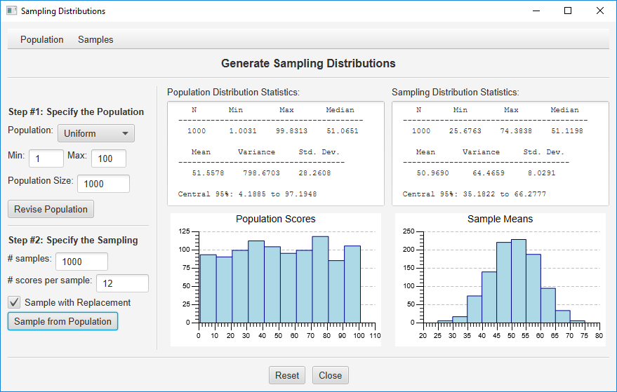
Note that the shape of the sampling distribution is more normal, the mean of the sample means will be about 50, and the standard deviation of the sample means will be about 8.3 This is consistent with what would be predicted by the Central Limit Theorum.
At any point, you can save your population or sample scores for more advanced analyses. Just use the menus at the top of the dialog and specify which scores you wish to output to a file or to your clipboard. Be aware of the potential for this to result in a large file and a processing delay if you are working with large populations or samples.
Other Population Distributions
Ok, Let’s work with a different random population distribution. Click the option button under “Use Random Population:” and you will see that you can generate a population of random scores from a uniform, normal, T, or Chi-Squared distribution. Choose “Chi-Squared,” specify 5 df, and then click the “Revise Population” button. Finally, use the sampling defaults and press the “Sample from Population” button:
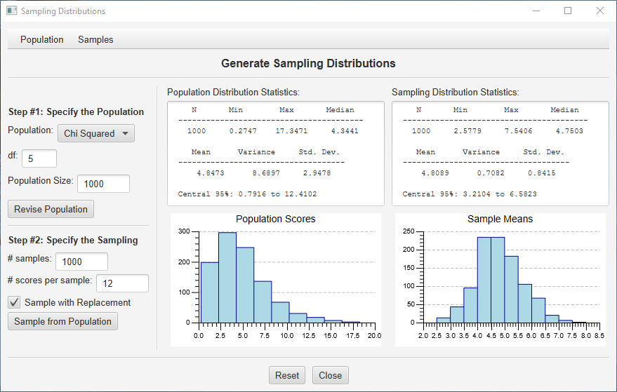
In the center column, you can see that the population is heavily skewed with a mean around 5. In the right column, you can see that the sampling distributions of the mean (computed from 12 scores from each random sample) is much more normally distributed. Again, this is exactly what you expect based on the Central Limit Theorum. Change the sample size from 12 to 32 and sample again. See the sampling distribution becoming even more normal?
Working with a Specific Population Distribution
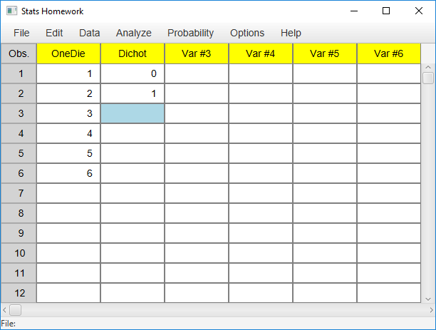
Here is an example I like to use in my statistics class. Imagine you are throwing a single die onto the table in front of you (I give my students dice to do this). Throw the die over and over and you get a number from 1 to 6. This is the population we will work with. In Stats Homework’s data manager, create a variable and enter the numbers 1 through 6:
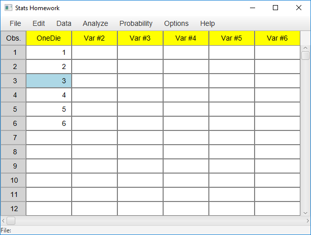
Now, in the sampling distribution routine’s dialog, click the option button for the population distribution and choose “Entered Data.” You will use a simple dialog to select this variable from the data manager. The descriptive statistics and histogram for this simple uniform population will be presented.
Now imagine that you are going to throw two dice at a time, and you will take the average of the dice each time (imagine my students all throwing dice on the table right now and writing down the means). To simulate this, specify a sample size of 2. Also, in order to create a very stable sampling distribution, specify 100,000 samples. Click “Sample from Population” and you will get this:
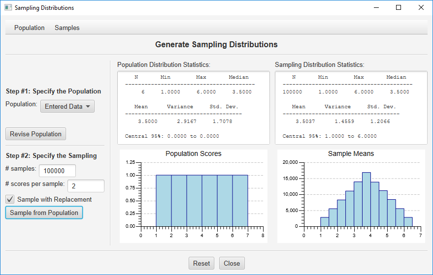
Isn’t that a pretty sampling distribution? Can you imagine how long it would take my students to throw the dice this many times?
Ok, one more example. Enter a new variable with two values, zero and one:
Choose this variable as your population, and then take samples of 6 from this population:
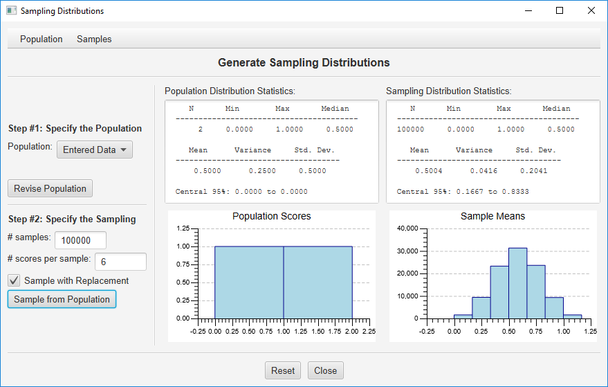
In this case, your sampling distribution is a binomial distribution where p = .50 and n = 6. If you would like p = .6, just enter 4 zeros and 6 ones as your population.
If you have some other population to work with, you can enter these data, read these data from a file, or paste them into the data manager from another editor. Again, you can save your population and sample data, along with a variety of sample statistics. You can save these data as a tab-delimited or as a CSV file, or you can copy these data to your clipboard. You can use a spreadsheet like Excel to open this file, or you can just paste the data from your clipboard.
Let me know if there are any options that you would like me to consider adding to this procedure.