Your homework problem:
You are interested in the relationship between one’s perception of how difficult a task is and one’s actual performance on that task. You have conducted an experiment with 24 participants who each performed an identical spatial-ability task. Each participant was randomly assigned to one of four treatment groups: six participants were led to believe that the task was of low difficulty, six were led to believe that the task was of moderate difficulty, six were led to believe that the task was of high difficulty, and six were told nothing about the difficulty of the task. Scores could range from 0 to 10, with higher scores indicating better performance on the task.
This study resulted in the following data:
| Low Difficulty |
Moderate Difficulty |
High Difficulty |
No Information |
| 6 | 8 | 4 | 4 |
| 7 | 7 | 1 | 5 |
| 4 | 5 | 2 | 5 |
| 5 | 8 | 4 | 6 |
| 4 | 9 | 6 | 8 |
| 6 | 7 | 3 | 6 |
Did the perceived level of task difficulty significantly affect the participants’ performance (alpha = .05)? If your analysis reveals a significant overall effect, then make sure to explore all possible mean differences with a post-hoc analysis (same alpha).
The appropriate test statistic for your study would be the value of the F statistic that would result from a One-Factor Between-Subjects Analysis of Variance (ANOVA):
![]()
The F statistic is equal to the ratio of the Mean Square Between-Groups divided by the Mean Square Within-Groups. k is equal to the number of groups, and N is equal to the total number of participants in your study.
Compute the test statistic. When we conduct an ANOVA, we typically construct a Source Table that details the sources of your variance and the corresponding degrees of freedom:
| Source | SS | df | MS | F |
| Between Groups: | ||||
| Within Groups: | ||||
| Total: |
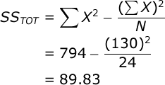
To facilitate your ANOVA, you should compute the following statistics: a) the sum of all scores (ΣX), the sum of all squared scores (ΣX²), the overall number of scores (N), and the number of scores in each treatment group (n). In our case, ΣX=130, ΣX²=794, N=24, and n=6. Compute these statistics for yourself now.
Also, you should compute the sum of scores (T) for each treatment group:
| Low Difficulty |
Moderate Difficulty |
High Difficulty |
No Information |
|
| T: | 32 | 44 | 20 | 34 |
Now, you are ready to conduct an Analysis of Variance. The Sum of Squares (SS) Total is equal to:
SS between-groups is equal to:

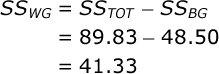
Again, T is equal to the sum of scores in a particular treatment group. The SS within-groups can be found by subtraction:
Add these values to your Source Table. The df Total is equal to the total number of scores minus one (N – 1). In our case this is: 24-1=23. The df Between-Groups is equal to the number of groups minus one (k – 1). In our case this is: 4-1=3. The df Within-Groups is equal to the number of participants minus the number of groups (N – k). In our case
this is: 24-4=20.
Each Mean Square (MS) is equal to the SS for that source divided by the df for that source. In our case, MS Between-Groups = 48.50 / 3 = 16.17, and MS Within-Groups = 41.333 / 20 = 2.067.
Now you are ready to compute your test statistic. F is equal to:
![]()
Here is your completed Source Table:
| Source | SS | df | MS | F |
| Between Groups: | 48.500 | 3 | 16.167 | 7.823 |
| Within Groups: | 41.333 | 20 | 2.067 | |
| Total: | 89.833 | 23 |
Conduct hypothesis test. In our study, the F statistic will have 3 and 20 df, and alpha = .05. If you look up the critical value of F in your table of critical values, you will see that if your obtained F is greater than 3.10, you would conclude that perceived task difficulty significantly affected actual task performance (i.e., that there exists one or more mean differences among the treatment group means).
Since the obtained F (7.82) is greater than the critical value for F (3.10), you would conclude that there was a significant overall effect of perceived task difficulty on performance.
Compute effect size. We will compute the overall effect size two ways. First let’s compute Eta Squared, which is very simple:
![]()
Eta Squared is an estimate of the proportion of variance in your dependent variable that can be accounted for by variation in your independent variable. However, the problem with Eta Squared is that it will systematically over-estimate the variance accounted for in your experiment; the smaller the sample size in your study, the more biased Eta Squared will be.
So, we typically prefer to compute an unbiased estimate of the variance accounted for.
Probably the best and most commonly used effect size statistic for a study like ours would be Omega Squared:
![]()
So, we would conclude that our manipulation of the perceived task difficulty accounted for 46% of the variance in our participants’ actual performance.
Post-Hoc testing. The F statistic provides us with an omnibus test of whether or not our independent variable affected our dependent variable. It does not, however, help us to understand the exact nature of this effect.
In our case, we know that there exists at least one significant mean difference among our treatment groups, but we have no idea at this point which particular mean difference might be significant. So, we should follow up our ANOVA with a post-hoc test. We will examine all pair-wise comparisons among our treatment groups and figure out which treatment group mean differences are statistically significant.
We will employ Tukey’s Honestly Significant Difference (HSD) test. This will reveal to us what would constitute a statistically significant mean difference between any two treatment group means, controlling alpha over the course of all of these comparisons. In our study, an Honestly Significant Difference would be equal to:
![]()
where q is equal to the Studentized Range Statistic and n is equal to the number of scores in each treatment group. In our case, we have 6 scores in each group. When alpha is equal to .05, you have 4 treatment groups, and you have 20 df within-groups, when you examine your table of critical values, you will find that the critical value of the Studentized Range Statistic for this study is equal to 3.958. So, the value of a significant mean difference in this study would be equal to:
![]()
Now, create a small table of the treatment group mean differences. Each value in this table is equal to the mean of the row group minus the mean of the column group:
| Treatment Group: | 1 | 2 | 3 | 4 |
| 1. Low Diff: | -2.00 | 2.00 | -0.33 | |
| 2. Mod Diff: | 4.00 | 1.67 | ||
| 3. High Diff: | -2.33 | |||
| 4. No Info: | ||||
| Group Mean: | 5.33 | 7.33 | 3.33 | 5.67 |
Then, compare the mean differences to your HSD. You will see that there are two significant pairwise comparisons among the treatment groups: the mean difference between the moderate-difficulty and the high-difficulty groups, and between the high-difficulty and the no-information groups.