Example homework problem:
Twenty five high school students complete a preparation program for taking the SAT test. We know that the overall average for SAT scores is 500 with a standard deviation of 100.
Here are the SAT scores from the 25 students who completed the SAT prep program:
434 694 457 534 720 400 484 478 610 641 425 636 454
514 563 370 499 640 501 625 612 471 598 509 531
Are these students’ SAT scores significantly greater than a population mean of 500 with a population standard deviation of 100? Note that the manufacturer’s claim and previous findings from studies like this would lead you to only consider the possibility that the prep program might have a positive effect on SAT scores. So, you will be conducting a one-tailed test. (alpha = .05).
If you would like help with the hand-written solution to this problem, click here.
Enter these data into the first column of Stats Homework’s data manager and rename this variable. Your screen should look like this:
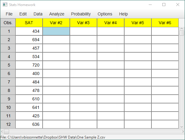
Make sure to double-check and save your data. To conduct your analysis, pull down the Analyze menu, choose One and Two Sample Tests, and then choose Z or T Test for One Sample.
You will be presented with a dialog window:
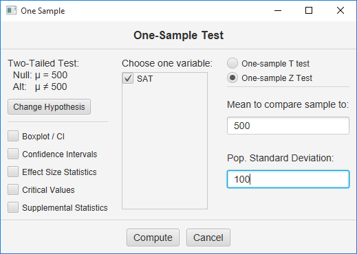
Check the variable that contains your data, click “One Sample Z Test,” and then enter 500 in the first blank and 100 in the second. Now, click the Change Hypothesis button. This dialog will appear:
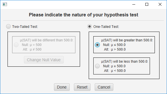
Click One-Tailed Test, and then click the top choice — indicating that you believe the SAT scores will average more than 500 if the null hypothesis is false. Click the Done button to return to this dialog:
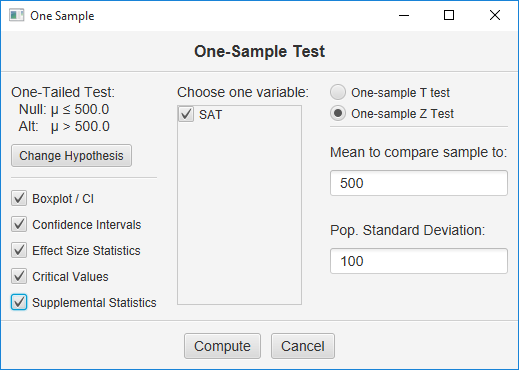
Verify that your null and alternative hypotheses have been specified correctly. Finally, check all the output options, and click the Compute button.
Basic Output
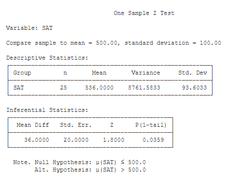
Compare Sample To. This is the population values that you are comparing your sample to with this Z test. Double-check to make sure that you entered the correct values (mean = 500 and sd = 100).
Descriptive Statistics. These basic statistics are described on the page for the explore procedure.
Inferential Statistics:
- Mean Diff (36.00): this is equal to the mean of your sample minus the population value that you entered.
- Std. Err. (20.00): this is the Standard Error of your Z Test. This will be equal to the standard deviation of your population divided by the square root of the sample size.
- Z (+1.80): this is the value of your test statistic. Z is equal to the mean difference divided by the standard error.
- p (2-tail) (.04): this is the chance probability / significance level for your Z test if you are conducting a one-tailed or directional hypothesis test.
Optional Outputs
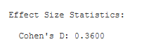
Cohen’s D: (.36): Cohen’s D is an effect-size estimate. It is equal to the mean difference divided by the standard deviation of the population. It standardizes the mean difference in terms of standard deviation units.
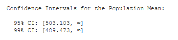
Confidence Intervals. You are given the 95% and 99% confidence intervals for the population mean, based on your sample mean.

Critical Values. These are the values from a statistical table of critical values for the Z test. In our case, we are conducting a one-tailed test with alpha = .05. So, we would compare the value of our obtained Z (1.80) to 1.645.
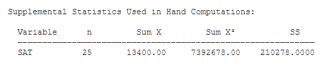
Supplemental Statistics Used in Hand Calculations. These are statistics that can be helpful if you would like to double check your hand-written computations.
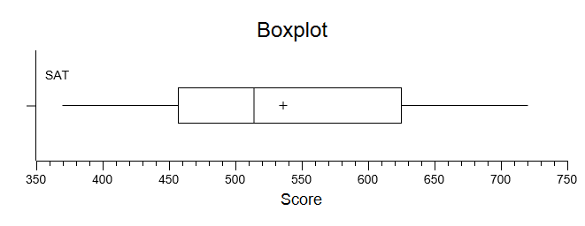
Box Plot. You can modify this plot, copy it to your clipboard, and save it to disk.