Your homework problem:
Aronson, Willerman, & Floyd (1966) investigated the impact of perceived competence on interpersonal liking. Participants were randomly assigned to one of four treatment conditions. In each, they listened to an audio recording of another student playing the part of a contestant on the ‘College Quiz Bowl’ game, where he would have to answer a number of interesting factual questions (similar to ‘Trivial Pursuit’). For half of the participants, the contestant was described as above average in every respect – he was an honor student, the editor of the campus yearbook, and a member of the school track team. For the other half of the participants, the contestant was described as average – he got average grades, he was a proofreader for the yearbook, and he tried out for the track team but did not compete. All the participants listened as the contestant played the Quiz Bowl game and answered many of the questions correctly (same male voice for all). For half of the participants, in the middle of one of his responses, the contestant spilled his coffee all over himself and sounded embarrassed about this accident. For the other half of the participants, the contestant did not spill his coffee. After the completion of the Quiz Bowl, the participants were asked to rate how much they liked the contestant – higher scores indicate greater interpersonal liking.
Here are some data similar to those collected by Aronson et al.:
| Ability Level |
Spilled Coffee | Did Not Spill Coffee |
| Average Ability | 2, 4, 5, 4, 3, 5 | 6, 4, 4, 5, 6, 3 |
| High Ability | 8, 6, 9, 7, 9, 8 | 6, 4, 5, 7, 3, 6 |
Did the manipulation of the contestant’s ability and whether or not he had an accident significantly affect the participants liking for him (alpha = .05)? Conduct a two-factor ANOVA to test the main effect for perceived competence of the contestant, the main effect for whether or not the contestant had an accident, and the interaction between the
two factors.
If you would like some help with your hand-written work, click here.
Separate Variable Approach
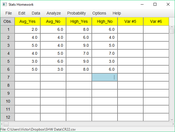
Enter these data into Stats Homework’s data manager as four separate variables, and rename the variables. It’s important that you name your variables carefully — each variable name indicates the level of perceived ability (‘Avg’ and ‘High,’ and the level of accident (‘Yes’ or ‘No’). Your screen should look like this:
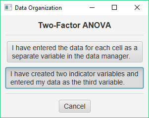
To conduct your analysis, pull down the Analyze menu, choose Analysis of Variance, and then choose Two-Factor ANOVA for Completely-Randomized Design. You will be presented with a dialog that asks you to specify the data-management approach that you are using:
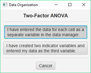
In this case, you should click the first button — you have entered your data as four separate variables. This will take you to the next dialog:
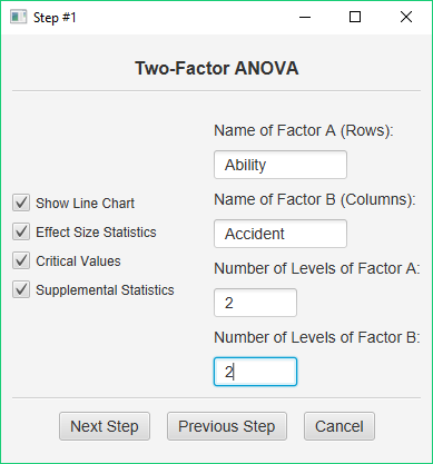 You should enter the names of your two factors — ‘Ability’ and ‘Accident.’ Then, enter the number of levels of each factor — 2 and 2. Finally, check all the output options and click Next Step. This brings up the next dialog:
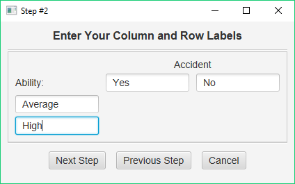
Here, you will label the levels of each factor. Enter ‘Yes’ and ‘No’ for your levels of Accident, and ‘Average’ and ‘High’ for your levels of Ability. Now, click Next Step. This brings up the last dialog:
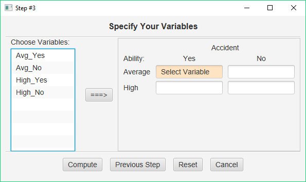
Here, you will specify how the variables that you entered into the data manager will be associated with the cells of your experimental design. You will click on a variable on the left, and then use the ‘===>’ button to move this variable to your design. So, you need to start with the variable that contains the data for the Ability = Average + Accident = Yes cell. When you are finished, this dialog should look like this:
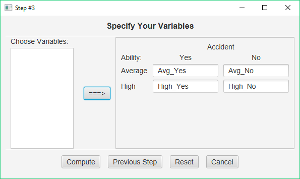
Now you can see why we entered our data into four variables in exactly this order — this makes it quite easy to specify our design for our analysis. In addition, you can now see why it is so important to name your variables in such a way that you indicate the levels of each of your independent variables. Pause here and study this design dialog to make sure that you have set up your analysis correctly.
Indicator Variable Approach
You will enter three variables — two indicator (independent) variables, and one dependent variable. You can use numeric or non-numeric indicator variables. Your data manager will look something like this:

Note that I prefer to use non-numeric indicator variables. This makes it clear which cell is which. You will see this clarity when you see the results for this analysis. When you call on the two-factor ANOVA procedure, you will start with this dialog:
Choose the second option — you have entered two indicator variables and one data variable. Now you will specify the design:
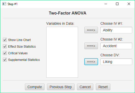
Move the indicator variable for Ability to the first blank, the indicator variable for Accident to the second blank, and the data variable to the third blank. Check all the options and click Compute. Did you notice that setting up the analysis this way was much easier? That’s because you did a lot of the work when you created your data — i.e., you specified the names of your factors and the labels for the factor levels. The program will figure out that you have a 2 X 2 Design by itself.
Basic Output
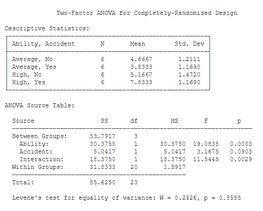
Descriptive Statistics. This table includes descriptive statistics for each treatment group / cell in your design.
ANOVA Source Table. This table details the result of the two-factor analysis of variance (ANOVA). This analysis partitions your variance into four sources: 1) the main effect for the first factor, 2) the main effect for the second factor, 3) the interaction between the factors, and 4) error (i.e., within-groups). Each variance component is associated with its own sum of squares (SS), degrees of freedom (df), and mean square (MS).
Each F statistic is equal to MS(effect) / MS(Within). Next to each F statistic is the corresponding value of p — the chance probability / significance level of the value of F.
Levene’s Test. One of the assumptions of your F test is that the treatment groups have equal variance. Levene’s W provides a formal test of this assumption. If the p value of W is less than .05, you would be concerned that your groups have unequal variance.
Optional Output
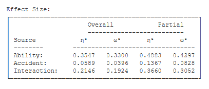 Effect Size. Eta Squared and Omega Squared describe the proportion of variance in your scores that can be attributed to your treatment effect. Omega Squared is an unbiased estimate of variance accounted for — i.e., it compensates for sample size. This table displays the values of overall Eta and Omega Squared, and partial Eta and Omega Squared. Discuss these effect size statistics with your instructor and decide which might be most appropriate for your analysis.
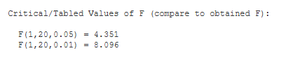
Critical Values. These are the values from a statistical table of critical values for the F test.
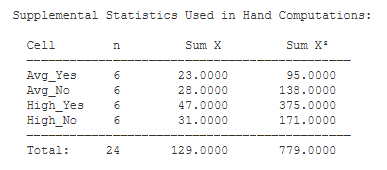
Supplemental Statistics. These are the preliminary statistics that you need to conduct this analysis by hand.
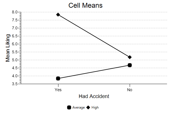
Line Chart. This graph can help you interpret a significant interaction, like in the case of this analysis. Note, for example, how there is not much of a difference in perceived liking when the contestant does not have an accident (i.e., the cell means above ‘No Acc’). However, there is a considerable difference in perceived liking when the contestant has an accident (i.e., the cell means above ‘Accident’). We especially like above-average people more than average people when they prove to be human by committing a blunder.
You can modify this chart in several ways — you can reverse the factors, resize the chart, and rescale the Y axis. Then, you can save the chart to disk or copy it to your clipboard.