Example homework problem:
Twenty participants were given a list of 20 words to process. The 20 participants were randomly assigned to one of two treatment conditions. Half were instructed to count the number of vowels in each word (shallow processing). Half were instructed to judge whether the object described by each word would be useful if one were stranded on a desert island (deep processing). After a brief distractor task, all subjects were given a surprise free recall task. The number of words correctly recalled was recorded for each subject. Here are the data:
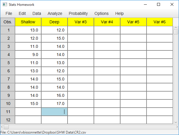
| Shallow Processing: | 13 | 12 | 11 | 9 | 11 | 13 | 14 | 14 | 14 | 15 |
| Deep Processing: | 12 | 15 | 14 | 14 | 13 | 12 | 15 | 14 | 16 | 17 |
Did the instructions given to the participants significantly affect their level of recall (alpha = .05)?
If you would like help with the hand-written solution for this problem, then click here.
Separate Variables Approach
Enter these data as two variables in Stats Homework’s data manager and rename the variables. Your screen should look like this:
Make sure to double-check and save your data. To conduct your analysis, pull down the Analyze menu, choose Tests for One or Two Samples, and then choose T Test for Independent Samples. Here is the user dialog you will work with:
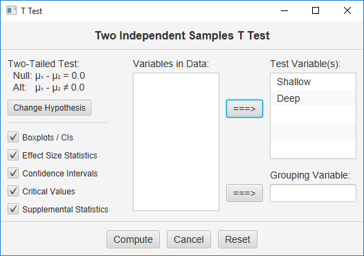
Move both of your variables to the “Test Variables” window, check all the output options, and click Compute.
Indicator Variable Approach
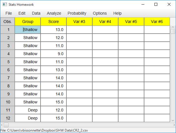
Enter the scores as one variable with 20 observations, and then create an indicator variable with two values to indicate which scores are from which sample. You can use a numeric or non-numeric indicator variable. Your screen should look something like this:
In this case, your user dialog will look like this:
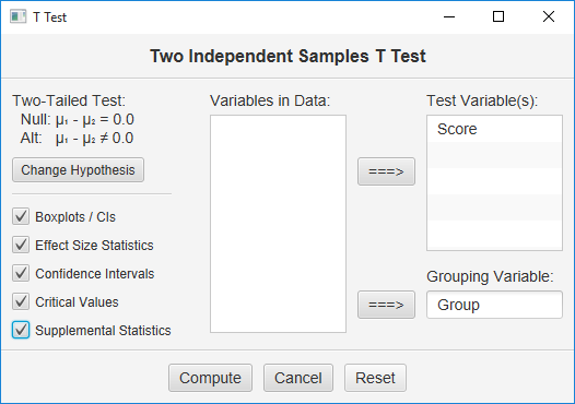
Move your indicator variable to the “Grouping Variable” box, and the variable containing your data to the “Test Variable” box. Click all the options and then click Compute.
Basic Output
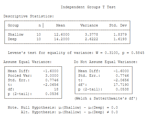
Descriptive Statistics. These basic statistics are described on the page for the explore procedure.
Levene’s Test for Inequality of Variance. This is a test of the equal-variance assumption of the t test. If this test reveals a significant difference in variance between your treatment groups (i.e., p < .05), then you would be advised to use the statistical result that assumes unequal variance.
Assume Equal Variance. This table lists the results of your t test if you assume that the groups have equal variance (i.e., Levene’s test is not significant).
- Mean Diff (-1.60): this is equal to the first mean minus the second mean.
- Pooled Var (3.00): this is equal to the Pooled Variance — a weighted average of the two sample variance (see hand-written
solution). - Std. Err. (0.77): this is the Standard Error of the mean difference (i.e., the denominator of the t statistic).
- t (-2.07): this is the value of the t test statistic. t is equal to the mean difference divided by the standard error of the difference.
- df (18): this is the df of the t test. df is equal to the total of the sample sizes minus 2.
- p (2-tail) (.05): this is the chance probability / significance level for your t test if you are conducting a two-tailed or non-directional
hypothesis test.
Do Not Assume Equal Variance. This table lists the results of your t test if you assume that the groups do not have equal variance (i.e., Levene’s test is significant). In this case, the df for the t test are estimated with Welch & Satterthwaite’s correction (17.72), which will change the resulting p value for this test.
Optional Outputs
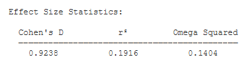
Effect Size Estimates.
- Cohen’s d (-0.92): Cohen’s D is an effect-size estimate. It is equal to the mean difference divided by the square root of the pooled variance. It standardizes the mean difference in terms of standard deviation units.
- r² (.19): r² is an effect-size estimate. It represents the proportion of variance in the dependent variable that is accounted for by the manipulation of the independent variable. It is equal to t² / (t² + df).
- Omega² (.14). Omega Squared is similar to r², in that it estimates the proportion of variance accounted for. However, it represents an unbiased estimate of variance accounted for — it accounts for sample size.
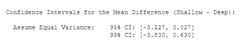
Confidence Intervals. You are given the 95% and 99% confidence intervals for the population mean difference, based on your sample mean difference. The 95% confidence interval tells you that, with 95% certainty, you would estimate the population mean difference to be between -3.23 and 0.03.
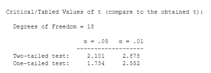
Critical Values. These are the values from a statistical table of critical values for the t test. In our case, we are conducting a two-tailed test with alpha = .05. So, we would compare the absolute value of our obtained t (2.07) to 2.101.
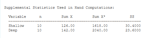
Supplemental Statistics Used in Hand Calculations. These are statistics that can be helpful if you would like to double check your hand-written computations.
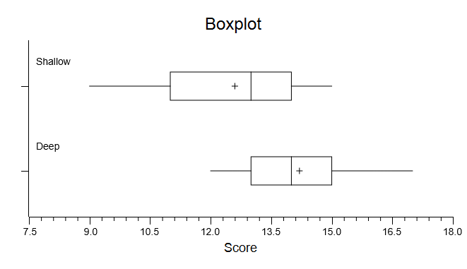
Box Plots. You can change these to graphical confidence intervals, change the scale, change the title and labels, save to disk, or copy to clipboard.