Example homework problem
You are an instructor, and you just gave your 15 students their first exam. You obtained the following scores — each score represents the percentage of exam items answered correctly:
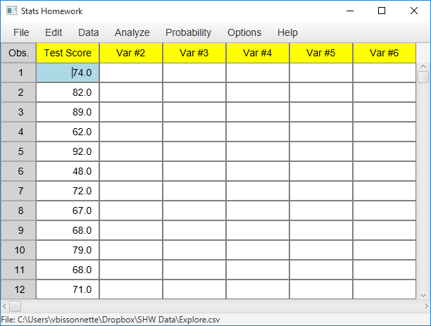
| Exam Score: | 74 | 82 | 89 | 62 | 92 | 48 | 72 | 67 | 68 | 79 | 68 | 71 | 79 | 80 | 69 |
Summarize these data with a variety of descriptive statistics that you are learning in your course. In particular, make sure to compute the mean, the variance, and the standard deviation of these scores.
If you would like some help with computing descriptive statistics by hand, click here.
Enter these data into the first column of Stats Homework’s data manager and give this variable a descriptive name. Your screen should look like this:
Always double-check and save your data. To conduct your analysis, pull down the Analyze menu and choose Explore Data. Here is the user dialog for this procedure:
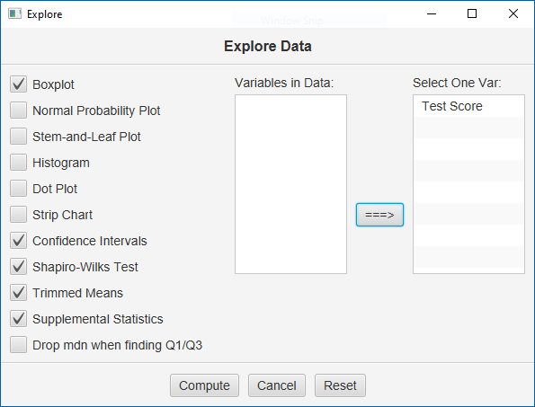
Move your variable to the window on the right, select all the optional output, select at least one graph, and click “Compute.”
Basic Output
Descriptive Statistics.
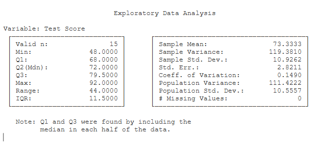
- Valid n (15): the number of scores in your sample.
- Min (48): the lowest score in your sample.
- Q1 (68): the first quartile.
- Q2 (72): the second quartile in your sample — the median.
- Q3 (79.50): the third quartile in your sample.
- Max (92): the highest score in your sample.
- Range (44): the largest score minus the smallest score.
- IQR: the inter-quartile range.
- Mean (73.33): the arithmetic mean of your sample; the average score (M = ΣX / n).
- Variance (119.38): the sample variance — the SS of your data divided by n – 1. (S² = SS / (n – 1)).
- Std. Dev. (10.93): the standard deviation — the square root of the sample variance (S = sqrt(SS / (n – 1)).
- Std. Err. (2.82): the standard error of the mean — the standard deviation divided by the square root of the sample size (SE = S / sqrt(n)).
- C.V. (0.15): the coefficient of variation — the standard deviation divided by the mean (CV = S / Mean).
Optional Outputs
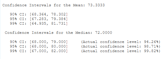 Confidence Intervals. Each confidence interval uses your sample to make a statement about what the mean of the population of all test scores might be. The first one tells you that with 95% certainty we know that the population mean of all test scores is between 67.28 and 79.38. The second group of confidence intervals include the median. Thus, with 98.7% confidence, we know that the population median is between 68 and 80.
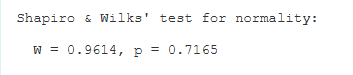 Distributional Statistics. Shapiro & Wilks’ test for normality: this test compares the shape of your sample distribution to that of the normal distribution. If the p value for this test is less than .05, this would suggest that your data are significantly non-normal. Many test statistics assume that your data are normally distributed. So, this test is a way to empirically check the assumption of normality in your data.
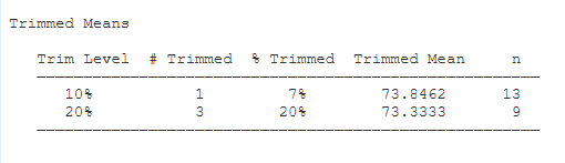
Trimmed Means. Here we have the means of your sample after trimming the most extreme values from the two tails of your sample. You will see the trimming goals — 10% and 20% — and the actual percentage trimmed from each tail of your sample — 7% and 20%. Finally, you will see the number of scores that were retained to compute the trimmed means.
Supplemental Statistics. These are statistics that can be helpful if you want to double-check your hand-written computations.
- Sum X (ΣX) (1100): the sum of the scores in your sample.
- Sum X² (ΣX²) (82338): the sum of the squared scores in your sample.
- SS (1671.33): the sum of squares of your sample — the sum of the squared deviations about the mean (SS = Σ(X – M)²).
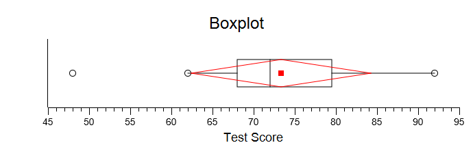
The Box Plot
- The middle of the box (72.0): the median of your sample.
- The “+” marker (73.33): the mean of your sample.
- The bottom and top of the box (68.0 and 79.50): the scores that take in the central 50% of your sample.
- The ends of the “whiskers” (62.0 and 92.0): the two most extreme scores that are not outliers.
- The “*” marker(s) (48.0): outliers (deviates more than 1 1/2 times the fourth spread from the upper or lower fourth).
- The (optional) red square (73.3): the sample mean.
- The (optional) red diamond (62.4 and 84.2): the sample mean minus and plus one standard deviation.
Make sure to explore the options for this plot. You can change the plot to a graphical confidence interval, and you can change a variety of features like the scale of the axis, and the title and labels.
If You Need Fewer Statistics
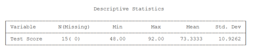
Stats Homework also includes a procedure for computing just the basic descriptive statistics. This procedure is especially helpful when you need the basic descriptive statistics on a number of variables. Pull down the Analyze menu and choose Descriptive Statistics. Here is the output screen that is produced: